3. Probability and Binomial Distributions of Data
Sign In
An error ocurred, try again later!
Chapter 9
3.
Probability and Binomial Distributions of Data
This lesson delves into the complexities of probability distribution, focusing on both experimental and theoretical aspects. It explains how to measure the variation of a probability distribution using metrics like variance and standard deviation. The text uses real-life examples, such as coin toss experiments, to illustrate these concepts. It also discusses the importance of these metrics in predicting outcomes and making informed decisions. For instance, the variance and standard deviation are used to understand how much an outcome will deviate from the expected value. The lesson also covers binomial distributions and their applications in various scenarios like gambling and customer behavior prediction. Overall, the lesson serves as a comprehensive guide for anyone looking to understand or apply probability distribution in real-world situations.
Show less Show more expand_more 


Lesson Settings & Tools
| | 13 Theory slides |
| | 8 Exercises - Grade E - A |
| | Each lesson is meant to take 1-2 classroom sessions |
Probability and Binomial Distributions of Data
Slide of 13
There are a variety of experiments whose outcomes can be reduced to success or failure. This lesson will explore how real-life situations that satisfy specific conditions can be modeled as binomial experiments. Additionally, methods of determining the probability of a certain number of successes in n binomial trials will be presented.
Catch-Up and Review
Here are a few recommended readings before getting started with this lesson.
Understanding Probability
Understanding Descriptive Measures
Understanding Types of Data
Other Recommended Readings
Explore
Share
Report error
Investigating Distributions Using Experiments
The Galton board is a device patented by Sir Francis Galton. It consists of a set of balls that are dropped from the top of the board. As the balls fall, they move to the left or right every time they bounce off of the pegs embedded in the board until they land in one of the bins at the bottom. Each path option has the same probability. 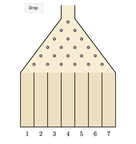 Based on the outcomes, try to ask the following questions.
- Which bins would be expected to collect the most balls?
- About how many balls are expected to land in each bin?
- How many paths branch out from each peg?
Discussion
Share
Report error
Analyzing the Probabilities of the Values of a Random Variable
A random variable assigns a numerical value to an outcome of a probability experiment. In many situations, it is important to know how likely it is that a random variable will take a specific value. This can be represented by listing or graphing the probability of each value of a random variable. This is called a probability distribution.
Concept
Share
Report error
Probability Distribution
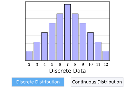
A probability distribution of a random variable X is a function that gives the probability of each outcome in the sample space. It can be represented by tables, equations, or graphs. A probability distribution needs to satisfy two conditions to be valid.
- The probability of each value of X is greater than or equal to 0 and less than or equal to 1.
- For a discrete variable, the sum of the probabilities of all possible values of X is 1.
Example
Consider the roll of a pair of standard dice. Let X be the random variable that represents the sum of the two dice. By the fundamental counting principle, since rolling each die has 6 possible outcomes, there are a total of 6* 6 = 36 possible results. Additionally, the possible values of X are integers from 2 to 12.
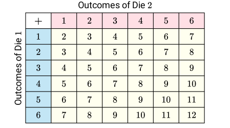
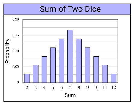
A table that represents the theoretical probability distribution of X will now be created. Frequencies represent the number of dice roll results that add up to the given values x of the random variable X. The frequency is divided by 36 to determine the theoretical probability of each outcome.
| X=Sum of Two Dice | ||
|---|---|---|
| x | Frequency | P(X=x) |
| 2 | 1 | 1/36≈ 0.028 |
| 3 | 2 | 2/36≈ 0.056 |
| 4 | 3 | 3/36≈0.083 |
| 5 | 4 | 4/36≈0.111 |
| 6 | 5 | 5/36≈0.139 |
| 7 | 6 | 6/36≈0.167 |
| 8 | 5 | 5/36≈0.139 |
| 9 | 4 | 4/36≈0.111 |
| 10 | 3 | 3/36≈0.083 |
| 11 | 2 | 2/36≈ 0.056 |
| 12 | 1 | 1/36≈ 0.028 |
Example
Share
Report error
Determine the Theoretical and Experimental Probability Distributions of a Coin Toss
Izabella is a big soccer fan. One weekend, she invited her friend Dylan to watch a world championship match together at her house. During the coin toss ceremony, Izabella asked Dylan about the number of heads they will obtain if they toss a fair coin four times.

Let X be a random variable that represents the number of heads in four coin flips. Help Izabella and Dylan solve the following problems and determine whether they can predict the number of times the experiment results in heads.
a Construct a table to describe the theoretical probability distribution of X.
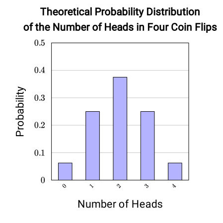
b Graph the theoretical probability distribution of X.
c Izabella and Dylan conducted an experiment of tossing the fair coin four times. They repeated this experiment 100 times and recorded the data in a tally sheet.
| Number of Heads, x | Tally | Frequency |
|---|---|---|
| 0 | |||| | | 6 |
| 1 | |||| |||| |||| |||| || | 22 |
| 2 | |||| |||| |||| |||| |||| |||| |||| || | 37 |
| 3 | |||| |||| |||| |||| |||| ||| | 28 |
| 4 | |||| || | 7 |
Use this data to find the experimental probability of each possible value of X.
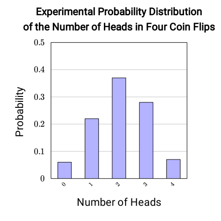
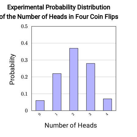
d Graph the experimental probability distribution of X.
Answer
a
| X=Number of Heads | |||||
|---|---|---|---|---|---|
| x | 0 | 1 | 2 | 3 | 4 |
| P(X=x) | 0.0625 | 0.25 | 0.375 | 0.25 | 0.0625 |
b
c
| X=Number of Heads | |||||
|---|---|---|---|---|---|
| x | 0 | 1 | 2 | 3 | 4 |
| P(X=x) | 0.06 | 0.22 | 0.37 | 0.28 | 0.07 |
d
Hint
a Think about the possible outcomes of tossing a coin four times. How can the outcomes be represented?
c Divide the frequency of each outcome by the total number of trials.
d The horizontal axis will represent the possible outcomes and the vertical axis will represent the probability of each outcome.
Solution
a The theoretical distribution of X will be determined by using a table. Observe the following simulation and think about the possible values for X. Keep in mind that there are exactly four coin flips.

| X=Number of Heads | |||||
|---|---|---|---|---|---|
| x | 0 | 1 | 2 | 3 | 4 |
| Possible Outcomes | T T T T | T T T H, T T H T, T H T T, H T T T | H H T T, H T T H, T T H H, H T H T, T H T H, T H H T | H H H T, H H T H, H T H H, T H H H | H H H H |
| Frequency | 1 | 4 | 6 | 4 | 1 |
Before calculating the theoretical probability of each value, find the total number of possible outcomes. Total: 1+4+6+4+1= 16 Now divide the frequency of each outcome by the total number of possibilities to calculate the probability P(X=x) that the random variable X takes the specific value x.
| X=Number of Heads | |||||
|---|---|---|---|---|---|
| x | 0 | 1 | 2 | 3 | 4 |
| Frequency | 1 | 4 | 6 | 4 | 1 |
| P(X=x) | 1/16 | 4/16=1/4 | 6/16=3/8 | 4/16=1/4 | 1/16 |
This table describes the theoretical probabilities associated with tossing a fair coin four times. Since only the theoretical probability is required, the Frequency
column can be skipped.
| X=Number of Heads | |||||
|---|---|---|---|---|---|
| x | 0 | 1 | 2 | 3 | 4 |
| P(X=x) | 0.0625 | 0.25 | 0.375 | 0.25 | 0.0625 |
b To graph the distribution, each possible outcome will be represented on the horizontal axis and the probability of each outcome on the vertical axis. Since only 0, 1, 2, 3, and 4 instances of heads are possible — it cannot appear 1.5 times out of 4 tosses, for example — the probability distribution is discrete and the bars on the graph will be separated.

c Consider the tally sheet prepared by Izabella and Dylan when conducting 100 trials of the experiment consisting of tossing a fair coin four times.
| Number of Heads, x | Tally | Frequency |
|---|---|---|
| 0 | |||| | | 6 |
| 1 | |||| |||| |||| |||| || | 22 |
| 2 | |||| |||| |||| |||| |||| |||| |||| || | 37 |
| 3 | |||| |||| |||| |||| |||| ||| | 28 |
| 4 | |||| || | 7 |
Calculate the experimental probability of each possible outcome by dividing its frequency by the total number of trials, 100.
| Number of Heads, x | Tally | Frequency | P(X=x) |
|---|---|---|---|
| 0 | |||| | | 6 | 6/100 |
| 1 | |||| |||| |||| |||| || | 22 | 22/100 |
| 2 | |||| |||| |||| |||| |||| |||| |||| || | 37 | 37/100 |
| 3 | |||| |||| |||| |||| |||| ||| | 28 | 28/100 |
| 4 | |||| || | 7 | 7/100 |
Since only the experimental probability is required, the Tally
and Frequency
columns can be skipped. Next, write the table horizontally.
| X=Number of Heads | |||||
|---|---|---|---|---|---|
| x | 0 | 1 | 2 | 3 | 4 |
| P(X=x) | 0.06 | 0.22 | 0.37 | 0.28 | 0.07 |
d Follow a similar method as in Part B to graph the probability distribution. Again, the horizontal axis will represent the possible values of X, while the vertical axis will represent the probability of each outcome.
Discussion
Share
Report error
Can the Experimental Distribution Estimate the Theoretical Distribution?
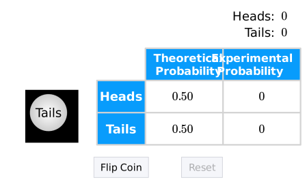
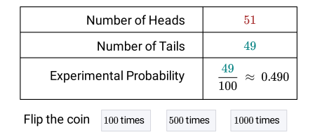
The expected value of a random variable X is the average of the possible outcomes of a random variable. It is used to describe the center of a probability distribution. For a discrete random variable, the expected value E(X) is given by the weighted mean.
E(X) = ∑ _(i=1)^n x_i * P(X=x_i)
In this formula, x_i represents a specific outcome, P(X=x_i) corresponds to the associated probability of x_i, and n is the number of all possible outcomes. According to the law of large numbers, when considering a sequence of random variables, its average tends to the expected value under specific conditions.
Rule
Share
Report error
Law of Large Numbers
Let X_1, X_2, ..., X_n be independent random variables with an identical probability distribution and S_n be the mean of the random variables. S_n=X_1+X_2+...+X_n/n The independence of random variables means that the events that different random variables take particular values are independent. If E(X_i)=μ represents the expected value of X_i, the law of large numbers states that S_n tends towards μ.
lim _(n → +∞) S_n=μ

Discussion
Share
Report error
How is the Variation of a Probability Distribution Measured?
The expected value is commonly used with a measure of variation such as the variance or standard deviation to determine how outcome will differ from the expected value.
Concept
Share
Report error
Variance of a Random Variable
The variance of a random variable describes how far from the expected value E(X) the outcomes of a random variable X are likely to be. To calculate the variance, begin by determining the deviation of each possible outcome x_i — the difference between x_i and E(X). Deviation ofx_i x_i-E(X) The variance is the total sum of the products of the deviation of each outcome and its corresponding probability P(X=x_i).
σ^2=Σ[[x_i-E(X)]^2* P(X=x_i)]
Concept
Share
Report error
Standard Deviation of a Random Variable
The standard deviation of a random variable is a measure of variation that describes how spread out the outcomes of a random variable X are from its expected value E(X). The standard deviation is represented by the Greek letter σ — read as sigma
— and is given by the square root of the variance of X.
σ=sqrt(Σ[[x_i-E(X)]^2* P(X=x_i)])
In this formula, x_i is a specific outcome and P(X=x_i) is the probability of x_i.
Example
Let X be the random variable representing the number of cars sold on a given day in a car dealership. The table below shows the probability distribution of X.
| x | 0 | 1 | 2 | 3 | 4 |
|---|---|---|---|---|---|
| P(X=x) | 1/15 | 3/15 | 6/15 | 3/15 | 2/15 |
E(X) = [x_1 * P(X=x_1)] + [x_2 * P(X=x_2)] + ... + [x_n * P(X=x_n)]
SubstituteValues
Substitute values
E(X) = 0( 1/15)+ 1( 3/15)+ 2( 6/15)+ 3( 3/15)+ 4( 2/15)
▼
Evaluate right-hand side
MoveLeftFacToNum
a*b/c= a* b/c
E(X) = 0/15+3/15+12/15+9/15+8/15
0/a=0
E(X) = 0+3/15+12/15+9/15+8/15
IdPropAdd
Identity Property of Addition
E(X) = 3/15+12/15+9/15+8/15
AddFrac
Add fractions
E(X) = 32/15
UseCalc
Use a calculator
E(X)=2.1333...
RoundDec
Round to 2 decimal place(s)
E(X) ≈ 2.13
| x_i | [x_i-E(X)]^2 | [x_i-E(X)]^2* P(X=x_i) |
|---|---|---|
| 0 | ( 0- 2.13)^2=4.5369 | 4.5364* 1/15≈ 0.3025 |
| 1 | ( 1- 2.13)^2=1.2769 | 1.2769* 3/15≈ 0.2554 |
| 2 | ( 2- 2.13)^2=0.0169 | 0.0169* 6/15≈ 0.0068 |
| 3 | ( 3- 2.13)^2=0.7569 | 0.7569* 3/15≈ 0.1514 |
| 4 | ( 4- 2.13)^2=3.4969 | 3.4969* 2/15≈ 0.4663 |
| Variance σ^2 | ≈ 1.1824 | |
Finally, calculate the square root of the variance to get the standard deviation of X.
Standard Deviation: sqrt(1.1824)≈ 1.09Variance vs Standard Deviation
The standard deviation is preferred over the variance because taking the square root of the variance gives the standard deviation the same units as X. This makes it possible to compare the possible outcomes relative to the expected value.Example
Share
Report error
Using Standard Deviation to Make a Decision
Izabella's aunt Magdalena owns a clothing store. She needs to increase stock in her shop and plans to invest $15 000 in one of the two collections that were offered to her by well-known brands. Each brand claims that they have a great expected rate of return. Their probability distributions are described below.
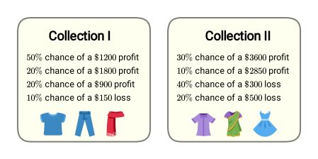
Dylan and Izabella want to help Magdalena make the best decision. They decided to use their recently acquired knowledge about the expected value and standard deviation of a probability distribution to analyze the offers. Help them answer the following questions and give the best advice to Magdalena.
a Pair each description with its corresponding measure.
{"type":"pair","form":{"alts":[[{"id":0,"text":"Expected Value of Collection I"},{"id":1,"text":"Expected Value of Collection II"},{"id":2,"text":"Standard Deviation of Collection I"},{"id":3,"text":"Standard Deviation of Collection II"}],[{"id":0,"text":"1125"},{"id":2,"text":"1145"},{"id":1,"text":"\u2248 516.36"},{"id":3,"text":"\u2248 1864.20"}]],"lockLeft":true,"lockRight":false},"formTextBefore":"","formTextAfter":"","answer":[[0,1,2,3],[0,2,1,3]]}
b Which investment should Izabella and Dylan advise Magdalena to choose?
{"type":"choice","form":{"alts":["Collection I","Collection II"],"noSort":false},"formTextBefore":"","formTextAfter":"","answer":0}
Hint
a The expected value is the total sum of the products of every possible value of the random variable and its corresponding probability.
b Compare the expected values and the standard deviations of the distributions.
Solution
a To match each description with its corresponding value, find the expected value and the standard deviation of each probability distribution one at a time.
Collection I
The expected value E(X) of a discrete random variable is given by the total sum of the products of every possible value x_i and its associated probability P(X=x_i). Let X represent the profit of the first collection. Note that each loss will be represented by a negative value.E(X)= [x_1* P(X=x_1)]+[x_2* P(X=x_2)]+...+[x_n* P(X=x_n)]
SubstituteValues
Substitute values
E(X)= 1200* 0.5+ 1800* 0.2+ 900* 0.2+( - 150)* 0.1
Multiply
Multiply
E(X)=600+360+180-15
AddSubTerms
Add and subtract terms
E(X)=1125
| x_i | [x_i-E(X)]^2 | [x_i-E(X)]^2* P(X=x_i) |
|---|---|---|
| 1200 | ( 1200- 1125)^2=5625 | 5625* 0.5= 2812.5 |
| 1800 | ( 1800- 1125)^2=455 625 | 455 625* 0.2= 91 125 |
| 900 | ( 900- 1125)^2=50 625 | 50 625* 0.2= 10 125 |
| -150 | ( -150- 1125)^2=1 625 625 | 1 625 625* 0.1= 162 562.5 |
| Sum of Values | 266 625 | |
The sum of the values of the last column represents the variance of the probability distribution. The standard deviation will be found by taking the square root of 266 625. Standard Deviation: sqrt(266 625)≈ 516.36
Collection II
Follow a similar procedure as before to calculate the expected value for Collection II.E(X)= [x_1* P(X=x_1)]+[x_2* P(X=x_2)]+...+[x_n* P(X=x_n)]
SubstituteValues
Substitute values
E(X)= 3600* 0.3+ 2850* 0.1+( -300)* 0.4+( - 500)* 0.2
Multiply
Multiply
E(X)=1080+285-120-100
AddSubTerms
Add and subtract terms
E(X)=1145
| x_i | [x_i-E(X)]^2 | [x_i-E(X)]^2* P(X=x_i) |
|---|---|---|
| 3600 | ( 3600- 1145)^2=6 027 025 | 6 027 025* 0.3= 1 808 107.5 |
| 2850 | ( 2850- 1145)^2=2 907 025 | 2 907 025* 0.1= 290 702.5 |
| -300 | ( -300- 1145)^2=2 088 025 | 2 088 025* 0.4= 835 210 |
| -500 | ( -500- 1145)^2=2 706 025 | 2 706 025* 0.2= 541 205 |
| Sum of Values | 3 475 225 | |
The square root of the variance will be calculated to find the standard deviation of the probability distribution of Collection II. Standard Deviation: sqrt(3 475 225)≈ 1864.20
Conclusion
The expected value and the standard distribution of each probability distribution have been calculated. The following table summarizes these measures.
| Measures of the Probability Distributions | ||
|---|---|---|
| Expected Value of Collection I | 1125 | |
| Expected Value of Collection II | 1145 | |
| Standard Deviation of Collection I | ≈ 516.23 | |
| Standard Deviation of Collection II | ≈ 1864.20 | |
b Consider the expected value of each distribution.
Expected Values Collection I: & E(X)=1125 Collection II: & E(X)=1145 The expected values do not give much information on their own because they are very close. This means that the expected profit of each collection is similar. Next, compare the standard deviations to determine which distribution has more variability. Standard Deviation Collection I: &σ≈ 516.36 Collection II: &σ≈ 1864.20 The standard deviation of Collection II is almost four times the that of Collection I, which implies that the expected value of Collection II will have about four times the variability of Collection I. Since Collection II is riskier, with a high chance for both gains and losses, Izabella and Dylan should advise Magdalena to invest in Collection I.
Discussion
Share
Report error
Binomial Experiments
The outcomes of many experiments can be reduced to two possibilities, success or failure. If two more conditions are satisfied, these experiments can be modeled by a binomial experiment.
Concept
Share
Report error
Binomial Experiment
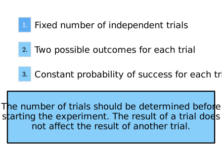
A binomial experiment is a probability experiment that has the following three properties.
- There is a fixed number of independent trials.
- Each trial has exactly two possible outcomes — success and failure.
- For each trial, the probability of success is constant.
Example
One of the most well-known examples of a binomial experiment is flipping a coin. There are only two possible outcomes, heads and tales. Either heads or tails could be considered a success, depending on the situation. The outcome of one toss does not impact the probability of the outcome of the next trial.
Extra
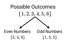
An Experiment Reducible to a Binomial ExperimentNote that many probability experiments can be reduced so that they satisfy the conditions of a binomial experiment. In case of rolling a die, there are six possible outcomes. However, they can be divided into two groups — even numbers and odd numbers, for example.

Example
Share
Report error
Classifying Whether Experiments Are Binomial
To better understand binomial experiments, Dylan and Izabella listed some examples of experiments. They want to determine whether the experiments can be modeled as binomial experiments. Which of these situations are examples of binomial experiments? 

 It cannot be known how many rolls it will take until a 3 comes up. Therefore the number of trials is not fixed. This means that this experiment does not represent a binomial experiment.
{"type":"multichoice","form":{"alts":["A coffee shop asks Mark to choose eight scratch-off cards randomly. Each card has a 25% chance of awarding a prize.","Asking 100 people their height.","Rolling a die until getting the number 3.","The probability of having blood type O is 0.4. Twenty people chosen at random are asked if their blood type is O."],"noSort":true},"formTextBefore":"","formTextAfter":"","answer":[0,3]}
Hint
Is there a fixed number of trials for each experiment? How many outcomes are possible? Does the probability of each outcome remain constant for each trial? Are trials independent?
Solution
Start by recalling the conditions that a binomial experiment should satisfy.
- There is a fixed number of independent trials.
- Each trial has exactly two possible outcomes — success and failure.
- For each trial, the probability of success is constant.
Analyze each situation one at a time to see if it follows all of the conditions of a binomial experiment.
The Scratch-off Cards
This situation has eight trials of selecting one scratch-off cards at random.
Each card could win a prize or not, which means there are two possible outcomes for each trial. Moreover, the probability of success, which is winning a prize, is 25 % or 0.25, for every card. P(Success)=0.25 Finally, the trials are independent because scratching one card does not affect the probability that any of the other cards reveals a prize. Therefore, this situation represents a binomial experiment.
Heights of 100 People
Note that height can vary for every people surveyed.
Because there are 100 possible answers, it is likely that more than 2 different outcomes will occur. This means that this situation does not represent a binomial experiment.
Rolling a Die
In this case, rolling a 3 can take only one or many more trials.Blood Type O
This situation has a fixed number of trials because it involves asking 20 people if their blood type is O.
Each trial has only two possible solutions, blood type O or another type. Moreover, the probability of having blood type O in each trial is 0.4, which represents the probability of success. P(Success)=0.4 Finally, because the answer of any person surveyed does not affect the probability that other people have O type blood, each trial is independent. This means that this situation is a binomial experiment.
Conclusion
All four situations have already been analyzed and the results are summarized in the following table.
| Experiment | Is It a Binomial Experiment? |
|---|---|
| The Scratch-off Cards | ✓ |
| Heights of 100 People | * |
| Rolling a Die | * |
| Blood Type O? | ✓ |
Discussion
Share
Report error
Probability of x Successes in n Binomial Trials
Because binomial experiments can simplify many complex situations, it is essential to determine how likely it is to obtain a specific number of successes out of n trials in a given experiment. Also, the expected value, or center of the distribution, will be presented.
Concept
Share
Report error
Binomial Distribution
The binomial distribution is the probability distribution that describes the number of successes x out of n binomial trials. The trials must satisfy three conditions.
- There is a fixed number of independent trials.
- Each trial has exactly two possible outcomes — success and failure.
- The probability of success is constant for each trial.
Let X be a random variable representing the total number of successes among n trials. The possible values of X are x=0, 1, 2, ..., n. The binomial probability formula can be used to determine the probability of x successes among n trials P(X=x).
P(X=x)=_nC_xp^xq^(n-x)
In this formula, _nC_x is the binomial coefficient and p and q are the probabilities of success and failure, respectively. Additionally, the expected value of X can be determined by the product of the number of trials n and the probability of success p.
E(X)=np
This means that the expected number of successes in n trials is given by np.
Example
Consider the experiment of drawing 1 card from a standard deck of cards with replacement.

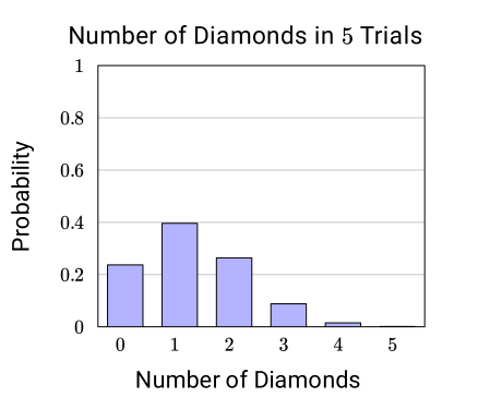
If drawing a diamond is considered a success, let X be the number of diamonds drawn. Since there are 13 diamond cards in a standard deck, the probability of success p in each trial will be 1352= 14. The probability of failure q will be 1- 14= 34. Suppose the experiment is repeated 5 times. Then, the binomial distribution with n= 5 can be determined. P(X= x)= _5C_x( 1/4)^x( 3/4)^(5- x) In this situation, the possible values of x are 0, 1, 2, 3, 4, and 5. The distribution of the random variable X can be obtained by evaluating this formula for each of these values.
| x | _5C_x(1/4)^x(3/4)^(5-x) | P(X=x)= _5C_x(1/4)^x(3/4)^(5-x) |
|---|---|---|
| 0 | _5C_0( 1/4)^0( 3/4)^(5- 0)=243/1024 | ≈ 0.237 |
| 1 | _5C_1( 1/4)^1( 3/4)^(5- 1)=405/1024 | ≈ 0.396 |
| 2 | _5C_2( 1/4)^2( 3/4)^(5- 2)=270/1024 | ≈ 0.264 |
| 3 | _5C_3( 1/4)^3( 3/4)^(5- 3)=90/1024 | ≈ 0.088 |
| 4 | _5C_4( 1/4)^4( 3/4)^(5- 4)=15/1024 | ≈ 0.015 |
| 5 | _5C_5( 1/4)^5( 3/4)^(5- 5)=1/1024 | ≈ 0.001 |
Extra
Deriving the Expected Value of a Binomial DistributionThe expected value E(X) of a discrete random variable X is given by the sum of the products of every possible value x_i of the variable and its corresponding probability P(X=x_i). E(X) = ∑ _(i=1)^n x_i * P(X=x_i)
Because the number of successes out of n trials can be x=0, 1, ..., n in a binomial experiment, the expected value of the binomial random variable can be simplified as follows.
E(X) = ∑ _(x=0)^n x * P(X=x)
The binomial probability formula gives that P(X=x) is equal to _nC_xp^xq^(n-x). This expression can be substituted into the simplified form of the expected value of a binomial distribution. E(X) = ∑ _(x=0)^n x * P(X=x) ⇓ E(X) = ∑ _(x=0)^n x * _nC_xp^xq^(n-x)
Note that when x is equal to 0, the expression x * _nC_xp^(x_i)q^(n-x)=0. This means that the first addend of the sum can be omitted and the first term of the sum is calculated for x=1.
E(X) = ∑ _(x=1)^n x * _nC_xp^xq^(n-x)
This formula can be manipulated to find the expected value of the binomial distribution.
Now, substitute y=x-1 and m=n-1.
If x=1, then y=0 If x=n, then y=n-1=m
The sum in the last expression can now be rewritten in terms of y and m by using this information.
Note that the sum corresponds to the Binomial Theorem. 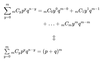 Next, recall that p+q=1 and that the powers of 1 are all equal to 1. Therefore, the sum will equal 1.
∑ _(y=0)^m _mC_y p^yq^(n-y)&=(p+q)^m &⇓ ∑ _(y=0)^m _mC_y p^yq^(n-y)&=1
Substituting this into the expression of the expected value results in the formula for the expected value of a binomial distribution.
Next, recall that p+q=1 and that the powers of 1 are all equal to 1. Therefore, the sum will equal 1.
∑ _(y=0)^m _mC_y p^yq^(n-y)&=(p+q)^m &⇓ ∑ _(y=0)^m _mC_y p^yq^(n-y)&=1
Substituting this into the expression of the expected value results in the formula for the expected value of a binomial distribution.
E(X) = ∑ _(x=1)^n x * _nC_x* p^xq^(n-x)
C(n,k)=n!/k! (n-k)!
E(X) = ∑ _(x=1)^n x * n!/x!(n-x)!* p^xq^(n-x)
▼
Rewrite
Write as a product
E(X) = ∑ _(x=1)^n x * n*(n-1)!/x*(x-1)!(n-x)!* p^xq^(n-x)
CancelCommonFac
Cancel out common factors
E(X) = ∑ _(x=1)^n x * n*(n-1)!/x*(x-1)!(n-x)!* p^xq^(n-x)
SimpQuot
Simplify quotient
E(X) = ∑ _(x=1)^n n*(n-1)!/(x-1)!(n-x)!* p^xq^(n-x)
Rewrite
Rewrite x as (x-1)+1
E(X) = ∑ _(x=1)^n n*(n-1)!/(x-1)!(n-x)!* p^((x-1)+1)q^(n-x)
SumInExponentOne
a^(1+m)=a*a^m
E(X) = ∑ _(x=1)^n n*(n-1)!/(x-1)!(n-x)!* p* p^(x-1)q^(n-x)
MovePartNumLeft
a* b/c=a*b/c
E(X) = ∑ _(x=1)^n n*(n-1)!/(x-1)!(n-x)!* p* p^(x-1)q^(n-x)
CommutativePropMult
Commutative Property of Multiplication
E(X) = ∑ _(x=1)^n np*(n-1)!/(x-1)!(n-x)! * p^(x-1)q^(n-x)
FactorOut
Factor out np
E(X) = np∑ _(x=1)^n ((n-1)!/(x-1)!(n-x)!)p^(x-1)q^(n-x)
Rewrite
Rewrite n-x as n-1-(x-1)
E(X) = np∑ _(x=1)^n ((n-1)!/(x-1)!((n-1)-(x-1))!)p^(x-1)q^((n-1)-(x-1))
E(X) = np∑ _(x=1)^n ((n-1)!/(x-1)!((n-1)-(x-1))!)p^(x-1)q^((n-1)-(x-1))
SubstituteValues
Substitute values
E(X) = np∑ _(y=0)^m (m!/y!(n-y)!)p^yq^(n-y)
C(n,k)=n!/k! (n-k)!
E(X) = np∑ _(y=0)^m _mC_y p^yq^(n-y)
E(X) = np∑ _(y=0)^m _mC_y p^yq^(n-y)
Substitute
∑ _(y=0)^m _mC_y p^yq^(n-y)= 1
E(X) = np* 1
MultByOne
a * 1=a
E(X) = np
Rule
Share
Report error
Binomial Probability
Let X be the random variable representing the number of successes in n binomial trials. The binomial probability P(X=x) can be calculated by using the following formula.
P(X=x)=_nC_xp^xq^(n-x)
In this formula, P(X=x) is the probability that the random variable X is equal to x, which means that there are exactly x successes. Additionally, p and q are the probabilities of success and failure, respectively, and _nC_x is the binomial coefficient.
Proof
This proof will begin by calculating the probability of obtaining a fixed sequence with x successes in n independent trials. The number of all possible sequences with x successes will then be calculated. Finally, joining the first and second parts will give the formula.
The Probability for a Fixed Sequence
Note that there are n independent trials, of which x are successes. This means that the difference between n and x gives the number of failures. rc Number of Succeses:& x Number of Failures:& n- x Furthermore, let p be the probability of success and q be the probability of failure in one individual trial. Therefore, by the Multiplication Rule of Probability and the fact that trials are independent, the probability of x successes is given by multiplying p by itself x times. Probability of xSuccesses: p* p* ... * p_(xtimes)=p^x Similarly, because there are n- x failures, the probability of n- x failures is given by multiplying q by itself n- x times. Probability of n- xFailures: q* q* ... * q_(n- xtimes)=q^(n- x) Therefore, the probability of getting exactly x successes and n- x failures is given by the product of p^x and q^(n- x) p^x q^(n- x) By the Commutative Property of Multiplication, any combination of p and q variables can be rearranged. Therefore, the expression is valid for any fixed sequence of x successes and n- x failures. However, note that this is the probability of only one of the possible sequences.
Finding the Total Number of Possible Sequences
Consider an experiment that consists of four independent trials. The sequences in which two successes S and two failures F occur are as follows. {S S F F, S F S F, S F F S, F S S F, F S F S, F F S S} Note that as long as two successes occur, the order of the outcomes is not important. This can be simplified by considering how many ways the two successes can be arranged within the four trials since the remaining trials will automatically be failures. In such a situation, the combination formula can be used._nC_r=n!/r!(n-r)!
SubstituteII
n= 4, r= 2
_4C_2=4!/2!( 4- 2)!
▼
Evaluate right-hand side
SubTerm
Subtract term
_4C_2=4!/2!*2!
Write as a product
_4C_2=4*3*2!/2!*2!
CrossCommonFac
Cross out common factors
_4C_2=4*3*2!/2!*2!
CancelCommonFac
Cancel out common factors
_4C_2=4*3/2!
Multiply
Multiply
_4C_2=12/2!
2!=2
_4C_2=12/2
CalcQuot
Calculate quotient
_4C_2=6
Getting the Binomial Probability
The probability of obtaining a fixed sequence of x successes out of n trials is given by the product of p to the power of x and q to the power of n- x. p^x q^(n- x) Moreover, there are _nC_x possible sequences with x successes. Therefore, by the Addition Rule of Probability, the probability P(X= x) of getting any of the possible sequences is given by adding the probability of getting one sequence _nC_x times. P(X=x)=p^x q^(n-x)+...+p^x q^(n-x)_(_nC_x times) ⇓ P(X=x)= _nC_x p^x q^(n-x)
Example
Share
Report error
Finding the Probability of Guessing Correctly on a Multiple-Choice Test
Dylan is taking a test that consists of five multiple-choice questions. Each question has five answer choices, only one of which is correct. He did not have time to study, so he decides to guess every answer.

{"type":"text","form":{"type":"math","options":{"comparison":"1","nofractofloat":false,"keypad":{"simple":false,"useShortLog":false,"variables":[],"constants":[]},"rendered":false},"text":" "},"formTextBefore":"P(X\u22653)\u2248","formTextAfter":"%","answer":{"text":["5.79"]}}
Hint
Consider using the Addition Rule of Probability.
Solution
To find the probability of guessing at least three answers correctly in a five question multiple-choice test, first, verify if this experiment satisfies the three conditions of a binomial experiment.
| Condition | Given Experiment | Is Satisfied? |
|---|---|---|
| There is a fixed number of independent trials. | There are five trials — five questions. | ✓ |
| Each trial has two possible outcomes. | The answer for each question is either correct or incorrect. | ✓ |
| The probability of success is constant for each trial. | The probability of guessing the correct answer for each question is 1 5= 0.2, where 5 is the number of options. | ✓ |
P(X=x)= _5C_x(0.2)^x(0.8)^(5-x)
Substitute
x= 3
P(X= 3)= _5C_3(0.2)^3(0.8)^(5- 3)
▼
Simplify right-hand side
C(n,k)=n!/k! (n-k)!
P(X=3)= (5!/3!(5-3)!)(0.2)^3(0.8)^(5-3)
SubTerms
Subtract terms
P(X=3)= (5!/3!* 2!)(0.2)^3(0.8)^2
Write as a product
P(X=3)= (5*4*3!/3!*2*1!)(0.2)^3(0.8)^2
CancelCommonFac
Cancel out common factors
P(X=3)= (5*4* 3!/3!*2*1!)(0.2)^3(0.8)^2
SimpQuot
Simplify quotient
P(X=3)= (5*4/2*1!)(0.2)^3(0.8)^2
▼
Evaluate right-hand side
1!=1
P(X=3)= (5*4/2*1)(0.2)^3(0.8)^2
Multiply
Multiply
P(X=3)= (20/2)(0.2)^3(0.8)^2
CalcQuot
Calculate quotient
P(X=3)= (10)(0.2)^3(0.8)^2
CalcPowProd
Calculate power and product
P(X=3)= 0.0512
| x | _5C_x(0.2)^x(0.8)^(5-x) | P(X=x)= _5C_x(0.2)^x(0.8)^(5-x) |
|---|---|---|
| 3 | _5C_3( 0.2)^3( 0.8)^(5- 3)=160/3125 | P(X= 3)= 0.0512 |
| 4 | _5C_4( 0.2)^4( 0.8)^(5- 4)=20/3125 | P(X= 4)= 0.0064 |
| 5 | _5C_5( 0.2)^5( 0.8)^(5- 5)=1/3125 | P(X= 5)≈ 0.00032 |
P(X≥3) = P(X=3)+P(X=4)+P(X=5)
SubstituteValues
Substitute values
P(X≥3)≈ 0.0512+0.0064+0.00032
AddTerms
Add terms
P(X≥3)≈ 0.05792
WritePercent
Convert to percent
P(X≥3)≈ 5.79 %
Example
Share
Report error
Finding the Number of Customers That Will Purchase Something
Izabella and Dylan are doing a fantastic job helping out at the clothing store. They noticed that the behavior of the customers can be modeled by a binomial experiment because there are two possible outcomes when customers enter the store — they either make a purchase or they do not.  Solve the following questions to help Izabella and Dylan find out if they can use their knowledge about binomial distributions in the store.
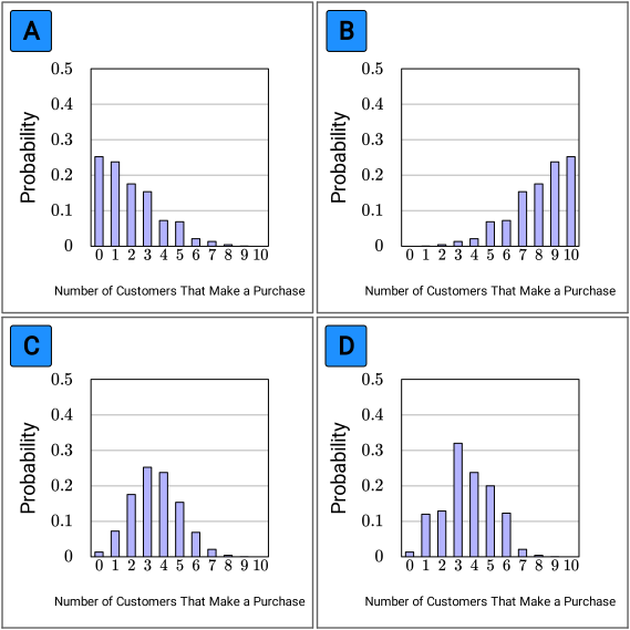 Based on past experience, Magdalena knows that the probability that a customer will make a purchase is about 0.35. Suppose that 10 customers will enter the store in the next hour. Which graph describes the probability associated with the number of customers who will make a purchase?
Let X be the random variable representing the number of customers that will make a purchase. The possible values of X are x=0, 1, ..., 10. Note that the probability of failure q will be 1- 0.35= 0.65. This information can now be input into the Binomial Probability Formula.
P(X=x)=_nC_xp^xq^(n-x) ⇓ P(X=x)=_(10)C_x( 0.35)^x( 0.65)^(10-x)
The binomial probability distribution will be determined by evaluating this formula for each of the possible values of x. In this case, the probability that none of the customers will make a purchase will be found first.
Similarly, the probability for the remaining values of x will be found.
The table can now be used to graph the probability distribution.
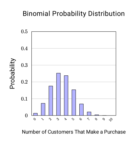 The graphed distribution corresponds to option C.
There is a probability of about 0.22 that exactly 3 out of 8 customers will make a purchase.
The graphed distribution corresponds to option C.
There is a probability of about 0.22 that exactly 3 out of 8 customers will make a purchase.
a Consider the following probability distributions.
{"type":"choice","form":{"alts":["A","B","C","D"],"noSort":true},"formTextBefore":"","formTextAfter":"","answer":2}
b Suppose the probability that one customer will make a purchase changes to 0.5. What is the probability that exactly 3 of the next 8 customers will make a purchase? Round to two decimal places.
{"type":"text","form":{"type":"math","options":{"comparison":"1","nofractofloat":false,"keypad":{"simple":false,"useShortLog":false,"variables":[],"constants":[]},"rendered":false},"text":" "},"formTextBefore":"P(X=3)\u2248","formTextAfter":null,"answer":{"text":["0.22"]}}
c Suppose that the store forecasts that 1500 customers will enter the store next month. If the probability that a customer will make a purchase is 0.35, find the expected number of customers that make a purchase next month.
{"type":"text","form":{"type":"math","options":{"comparison":"1","nofractofloat":false,"keypad":{"simple":false,"useShortLog":false,"variables":[],"constants":[]},"rendered":false},"text":" "},"formTextBefore":"E(X)=","formTextAfter":null,"answer":{"text":["525"]}}
Hint
a Begin by identifying the conditions of a binomial experiment.
b Evaluate the Binomial Probability Formula at x=3.
c The expected value is given by the product of the number of trials and the probability of success.
Solution
a Notice that the graphs each consider ten customers, so there are ten trials. In each trial, a success is that a customer makes a purchase. Start by identifying whether this experiment follows the three conditions of a binomial experiment.
| Condition | Given Experiment | Is Satisfied? |
|---|---|---|
| There is a fixed number of independent trials. | There are 10 trials — the 10 customers that will enter the store. | ✓ |
| Each trial has two possible outcomes. | Whether a customer makes a purchase or not. | ✓ |
| The probability of success is constant for each trial. | There is a 0.35 probability that a customer will make a purchase. | ✓ |
P(X=x)=_(10)C_x(0.35)^x(0.65)^(10-x)
Substitute
x= 0
P(X=0)=_(10)C_0(0.35)^0(0.65)^(10- 0)
▼
Evaluate right-hand side
C(n,k)=n!/k! (n-k)!
P(X=0)=(10!/0!(10-0)!)(0.35)^0(0.65)^(10-0)
SubTerms
Subtract terms
P(X=0)=(10!/0!(10!))(0.35)^0(0.65)^(10)
0!=1
P(X=0)=(10!/1(10!))(0.35)^0(0.65)^(10)
MultByOne
a * 1=a
P(X=0)=(10!/10!)(0.35)^0(0.65)^(10)
QuotOne
a/a=1
P(X=0)=1(0.35)^0(0.65)^(10)
CalcPowProd
Calculate power and product
P(X=0)=0.013462...
RoundDec
Round to 4 decimal place(s)
P(X=0)≈ 0.0135
| x | _(10)C_x(0.35)^x(0.65)^(10-x) | P(X=x)= _(10)C_x(0.35)^x(0.65)^(10-x) |
|---|---|---|
| 0 | _(10)C_0( 0.35)^0( 0.65)^(10- 0) | P(X= 0)≈ 0.01346 |
| 1 | _(10)C_1( 0.35)^1( 0.65)^(10- 1) | P(X= 1)≈ 0.07249 |
| 2 | _(10)C_2( 0.35)^2( 0.65)^(10- 2) | P(X= 2)≈ 0.17565 |
| 3 | _(10)C_3( 0.35)^3( 0.65)^(10- 3) | P(X= 3)≈ 0.25222 |
| 4 | _(10)C_4( 0.35)^4( 0.65)^(10- 4) | P(X= 4)≈ 0.23767 |
| 5 | _(10)C_5( 0.35)^5( 0.65)^(10- 5) | P(X= 5)≈ 0.15357 |
| 6 | _(10)C_6( 0.35)^6( 0.65)^(10- 6) | P(X= 6)≈ 0.06891 |
| 7 | _(10)C_7( 0.35)^7( 0.65)^(10- 7) | P(X= 7)≈ 0.02120 |
| 8 | _(10)C_8( 0.35)^8( 0.65)^(10- 8) | P(X= 8)≈ 0.00428 |
| 9 | _(10)C_9( 0.35)^9( 0.65)^(10- 9) | P(X= 9)≈ 0.00051 |
| 10 | _(10)C_(10)( 0.35)^(10)( 0.65)^(10- 10) | P(X= 10)≈ 0.00003 |
b In order to find the probability that exactly 3 out of 8 customers will make a purchase, P(X=3) needs to be found. In this case, the number of trials is 8, the probability of success is 0.5, and the probability of failure is 0.5. Use the Binomial Probability Formula again.
P(X=x)=_8C_x(0.5)^x(0.5)^(8-x)
Substitute
x= 3
P(X= 3)=_8C_3(0.5)^3(0.5)^(8- 3)
▼
Evaluate right-hand side
C(n,k)=n!/k! (n-k)!
P(X=3)=(8!/3!*(8-3)!)(0.5)^3(0.5)^(8-3)
SubTerms
Subtract terms
P(X=3)=(8!/3!*5!)(0.5)^3(0.5)^5
MultPow
a^m*a^n=a^(m+n)
P(X=3)=(8!/3!*5!)(0.5)^8
SplitIntoFactors
Split into factors
P(X=3)=(8*7*6*5!/3*2*1*5!)(0.5)^8
CancelCommonFac
Cancel out common factors
P(X=3)=(8*7*6*5!/3*2*1*5!)(0.5)^8
SimpQuot
Simplify quotient
P(X=3)=(8*7*6/3*2*1)(0.5)^8
Multiply
Multiply
P(X=3)=(336/6)(0.5)^8
CalcQuot
Calculate quotient
P(X=3)=56(0.5)^8
CalcPowProd
Calculate power and product
P(X=3)=0.21875
RoundDec
Round to 2 decimal place(s)
P(X=3)≈ 0.22
c Magdalena estimates that about 1500 customers will enter the store next month. Let X be the random variable representing the number of customers that will make a purchase. Since this random variable follows a binomial distribution, its expected value is given by the product of the number of trials n and the probability of success p.
Expected Value ofX E(X) = np In this case, the number of trials n is 1500 and the probability of success is 0.35. The expected number of customers who will make a purchase next month can be determined with this information. E(X)= 1500* 0.35 ⇕ E(X)=525 Therefore, 525 customers are expected to make a purchase next month.
Closure
Share
Report error
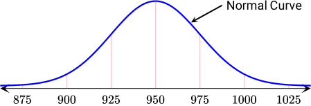
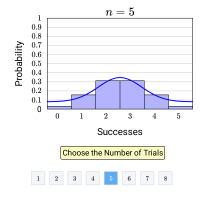
Normal Approximation to the Binomial Distribution
The binomial distribution is a discrete distribution that helps find the probability of the number of successes in a binomial experiment. In some cases, these calculations may be too complex. In such instances, a continuous distribution called normal distribution might approximate the calculations.
Probability and Binomial Distributions of Data
Exercise 3.1
A poll of Americans determined that 80 % prefer living in the countryside. Ten American people are chosen randomly. The probability that at least x of the people chosen want to live in the countryside is about 0.678 or 67.8 %

{"type":"text","form":{"type":"math","options":{"comparison":"1","nofractofloat":false,"keypad":{"simple":true,"useShortLog":false,"variables":[],"constants":[]},"rendered":false},"text":" "},"formTextBefore":"x=","formTextAfter":null,"answer":{"text":["8"]}}
security
report
code
security
report
code
We are asked to find the value of x that makes the probability that at least x out of the 10 polled Americans prefer living in the countryside about 0.678. We are given that 80 % of Americans prefer living in the countryside. This means that the remaining 100-80=20 % of Americans do not prefer to live in the countryside.
| Poll | |
|---|---|
| Americans who prefer to live in the countryside | 80 %=0.8 |
| Americans who do not prefer to live in the countryside | 20 %=0.2 |
We can note that randomly questioning Americans can be modeled as a binomial experiment, with success being that they prefer living in the countryside and failure that they do not. Considering the results of the poll, we can state the probability of success and failure as p= 0.8 and q= 0.2, respectively.
| Event | Probability | |
|---|---|---|
| Success | Success: American prefers to live in the countryside | p= 0.8 |
| Failure | Failure: American does not prefer to live in the countryside | q= 0.2 |
To determine the value of x, we will first calculate the probabilities that 0, 1, ..., 9, or 10 of the chosen people answered that they prefer living in the countryside. This means that we need to find the probabilities of getting exactly 0 successes, 1 success, and so on. To do so, let's use the Binomial Probability Formula. P(X=x)= _nC_x p^x q^(n-x) Because in this case 10 people are randomly chosen, the number of trials is 10. This means that we can subsitute n= 10, p= 0.8, and q= 0.2 into the formula. P(X=x)= _(10)C_x 0.8^x 0.2^(10-x) Now we will calculate the probability that X takes the values of x=0, 1, ..., 10. Before evaluating the formula, we can get the values of _(10)C_x using the first ten rows of Pascal's Triangle.
Using this information, let's calculate the probabilities.
| Number of Successes, x | P(X=x)= _(10)C_x0.8^x 0.2^(10-x) | P(X=x) Simplified | P(X=x) Evaluation |
|---|---|---|---|
| 0 | _(10)C_00.8^0 0.2^(10- 0) | 1* 1* 0.2^(10) | P(0)≈ 0.0000 |
| 1 | _(10)C_10.8^1 0.2^(10- 1) | 10* 0.8* 0.2^9 | P(1)≈ 0.0000 |
| 2 | _(10)C_20.8^2 0.2^(10- 2) | 45* 0.8^2* 0.2^8 | P(2)≈ 0.0001 |
| 3 | _(10)C_30.8^3 0.2^(10- 3) | 120* 0.8^3* 0.2^7 | P(3)≈ 0.0008 |
| 4 | _(10)C_40.8^4 0.2^(10- 4) | 210* 0.8^4* 0.2^6 | P(4)≈ 0.0055 |
| 5 | _(10)C_50.8^5 0.2^(10- 5) | 252* 0.8^5* 0.2^5 | P(5)≈ 0.0264 |
| 6 | _(10)C_60.8^6 0.2^(10- 6) | 210* 0.8^6* 0.2^4 | P(6)≈ 0.0881 |
| 7 | _(10)C_70.8^7 0.2^(10- 7) | 120* 0.8^7* 0.2^3 | P(7)≈ 0.2013 |
| 8 | _(10)C_80.8^8 0.2^(10- 8) | 45* 0.8^8* 0.2^2 | P(8)≈ 0.3020 |
| 9 | _(10)C_90.8^9 0.2^(10- 9) | 10* 0.8^9* 0.2^1 | P(9)≈ 0.2684 |
| 10 | _(10)C_(10)0.8^(10) 0.2^(10- 10) | 1* 0.8^(10)* 1 | P(10)≈ 0.1074 |
Next, we can start looking for the value of x. Consider that the probability of at least x out of the 10 questioned people preferring living in the countryside is equal to the probability that at least x successes occurred. The probability that at least x success occurred is equal to the sum of the probabilities of x, x+1, ..., and 10 successes occurred. P(At leastxsuccesses)= P(X = x) + P(X = x + 1) + ... + P(X = 10) We want to find x for which this sum is about 0.678. We will continue calculating this sum for x=10, 9, ..., 0 until we find the right value.
| At least x successes | P(At leastxsuccesses) | Substitute | Evaluate |
|---|---|---|---|
| At least 10 successes | P(10) | 0.1074 | ≈ 0.107 |
| At least 9 successes | P(9)+P(10) | 0.2684 +0.1074 | ≈ 0.376 |
| At least 8 successes | P(8)+P(9)+P(10) | 0.3020+0.2684+0.1074 | ≈ 0.678 |
| ... | ... | ... | ... |
When we have reached the probability of at least 8 successes, we got the value we are looking for. Therefore, the value of x is 8. This means that with a probability of 0.678, 8 of the people chosen want to live in the countryside.
security
report
code
Probability and Binomial Distributions of Data
Recommended exercises
To get personalized recommended exercises, please login first.
Loading content
≤
>
■2
■▢
e▢
7
8
9
×
÷■1
=
=
√▢
▢√
∫▢▢
4
5
6
+
−
≤
<
log
ln
log▢
1
2
3
()
∣
sin
cos
tan
0
.
π
x
y
Loading content