{{ tocSubheader }}
{{ 'ml-label-loading-course' | message }}
An error ocurred, try again later!
Chapter {{ article.chapter.number }}
{{ article.number }}.
{{ article.displayTitle }}
{{ article.intro.summary }}
Show less Show more expand_more Lesson Settings & Tools
| | {{ 'ml-lesson-number-slides' | message : article.intro.bblockCount }} |
| | {{ 'ml-lesson-number-exercises' | message : article.intro.exerciseCount }} |
| | {{ 'ml-lesson-time-estimation' | message }} |
When discussing trigonometric functions such as the sine, cosine, and tangent functions, it is natural to consider their reciprocal functions.
| Trigonometric Function | Reciprocal Trigonometric Function |
|---|---|
| y=sinx | y=sinx1 |
| y=cosx | y=cosx1 |
| y=tanx | y=tanx1 |
This lesson will explore the graphs of these reciprocal trigonometric functions.
Catch-Up and Review
Here are a few recommended readings before getting started with this lesson.
Challenge
Communication Tower
A massive communication tower is anchored to the ground with wires.

y=5cscθ
Here, θ is the measure of the angle formed by the wire and the ground. Graph the given function to find the length of the wire that makes an angle of 4π radians with the ground. Round the answer to the nearest integer. {"type":"text","form":{"type":"math","options":{"comparison":"1","nofractofloat":false,"keypad":{"simple":true,"useShortLog":false,"variables":[],"constants":[]},"rendered":false},"text":"<span class=\"katex\"><span class=\"katex-html\" aria-hidden=\"true\"><\/span><\/span>"},"formTextBefore":null,"formTextAfter":"meters","answer":{"text":["7"]}}
Explore
Exploring the Graphs of the Cosine and Sine Functions, and Their Quotient
In the diagram, the graphs of the functions y=sinx, y=cosx, and y=sinxcosx can be seen.
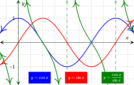 Consider the graph of y=sinxcosx. How is it different from the other two graphs? What happens in the graph of y=sinxcosx when sinx=0?
Discussion
The Cotangent Function
Let P be the point of intersection of the terminal side of an angle in standard position and the unit circle. The cotangent function, denoted by cot, is defined as the ratio of the x-coordinate to the y-coordinate of P.
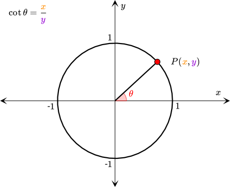
cotθ=sinθcosθ
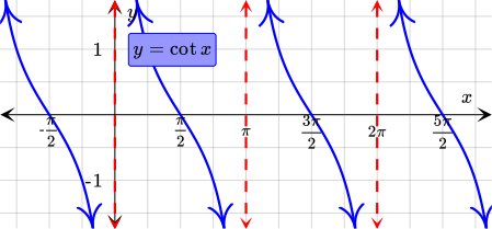
Since division by 0 is not defined, the graph of the parent cotangent function y=cotx has vertical asymptotes where sinx=0. This means that the graph has vertical asymptotes at every multiple of π. The graph of y=cotx can be drawn by making a table of values.
Consider now the general form of a cotangent function.
y=acotbx
Here, a and b are non-zero real numbers and x is measured in radians. The properties of the cotangent function are stated below.
| Properties of y=acotbx | |
|---|---|
| Amplitude | No amplitude |
| Number of Cycles in [0,2π] | 2∣b∣ |
| Period | ∣b∣π |
| Domain | All real numbers except multiples of ∣b∣π |
| Range | All real numbers |
Method
Graphing a Cotangent Function
Recall the format of a cotangent function.
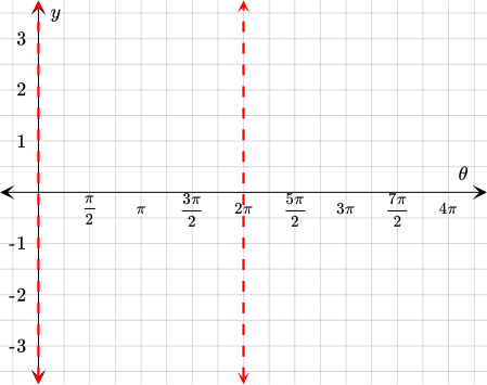
y=acotbθ
Here, a and b are non-zero real numbers and θ is measured in radians. The values of a and b can be used to graph the function. Consider an example function.
y=3cot21θ
In this function, a=3 and b=21. To sketch one cycle of a cotangent curve, its asymptotes and three points can be used. As with other trigonometric functions, there are five elements that are equally spaced through one cycle. The asymptote-point-zero-point-asymptote pattern is helpful for graphing this function. Four steps will be followed.
1
Find the Period and Cycle
expand_more The period of a cotangent function is the quotient of π and ∣b∣.
Period∣b∣π⇒∣∣∣21∣∣∣π=2π
The period of this function is 2π. This means that one cycle goes from 0 to 2π. 2
Graph the Asymptotes
expand_more Asymptotes occur at the end of each cycle. Therefore, the given function has asymptotes at θ=0 and θ=2π.
3
Divide the Period and Locate Points
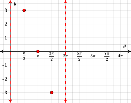
expand_more Divide the period into fourths and locate the three equidistant points between the asymptotes. The period for this function goes from 0 to 2π, so a table of values will be made for θ=2π, θ=π, and θ=23π.
| θ | 3cot(21θ) | y |
|---|---|---|
| 2π | 3cot(21⋅2π) | 3 |
| π | 3cot(21⋅π) | 0 |
| 23π | 3cot(21⋅23π) | -3 |
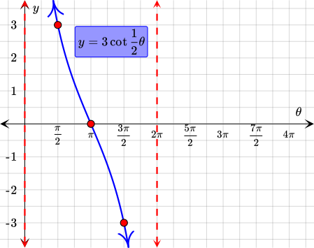
The points found in the table are (2π,3), (π,0), and (23π,-3).
4
Draw the Graph
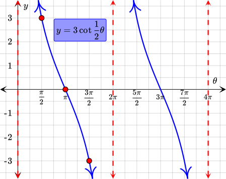
expand_more Finally, the points can be connected with a smooth curve to draw the graph for one cycle.
Once the graph for one cycle is drawn, it can be replicated as many times as desired to draw more cycles. Here, another cycle is graphed.
Extra
Alternative MethodAlternatively, the graph of a cotangent function can be drawn by considering the graphs of the sine and cosine functions. To show this method, the graph of the parent cotangent function will be drawn.
y=cotx
To draw the graph by using this method, five steps will be followed.
1
Graph the Sine and Cosine Functions
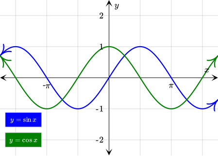
expand_more Start by drawing the graphs of the the sine and cosine functions on the same coordinate plane.
2
Draw the Asymptotes
expand_more 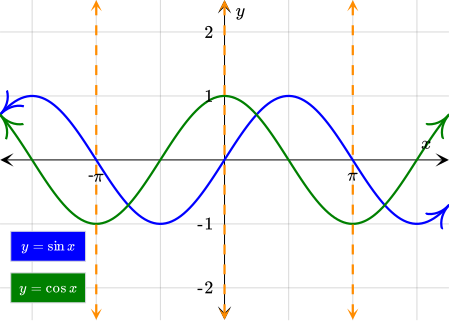
3
Plot Two Zeros
expand_more Since the cotangent of an angle is the ratio of the cosine to the sine of the angle, the cotangent function and the cosine function have the same zeros.
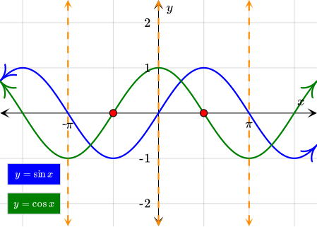
cotθ=0⇔cosθ=0
Therefore, the x-intercepts of the cotangent function occur when cosx=0.
4
Plot More Points on the Curve
expand_more By definition, the cotangent function is 1 when the cosine and the sine have the same value. This happens at their points of intersection. Therefore, the y-value of the cotangent function will be 1 at the x-coordinate of these points.
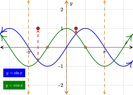 Similarly, the output of the cotangent function is -1 when the sine and the cosine function have opposite values.
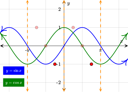
5
Draw the Graph
expand_more Finally, two cycles of the cotangent function can be graphed by connecting the marked points.
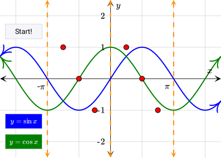 It is seen that the period of the cotangent function is π. Since each branch comes from positive infinity towards negative infinity, the cotangent function has no amplitude and its range is all real numbers.
Example
Tanabata Trees and a Cotangent Function
Tanabata is a Japanese festival that celebrates two mythical lovers separated by the Milky Way. A Tanabata tree is a type of tree on which people hang wishes written on paper during Tanabata. Ramsha is starting a Tanabata garden in her backyard. She realized that two of the Tanabata trees follow the path of one cycle of a cotangent function. 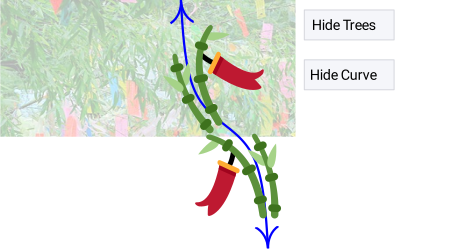 After doing some calculations, she found the equation of the curve that these trees follow.
External credits: Kumiko
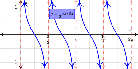
y=21cot2x
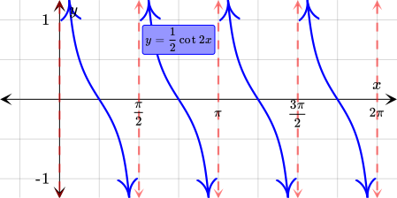
Draw the graph of the function for values of x between 0 and 2π.
Answer
Hint
Find the period and cycle, then graph the asymptotes and plot some points. Finally, sketch the curve.
Solution
To graph a cotangent function, the first step is to calculate the period. To do so, consider the general form of a cotangent function and the given function.
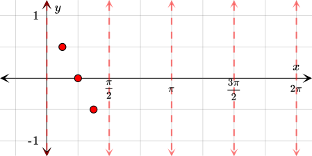
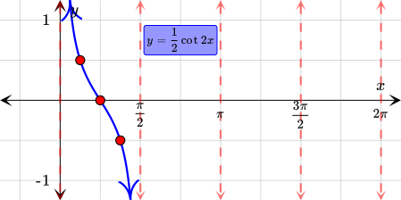
General Form:Given Function: y=acotbx y=21cot2x
Here, a=21 and b=2. The period of the function is the quotient of π and ∣b∣.
Period ∣b∣π⇒2π
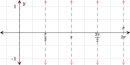
The period of the function is 2π. This means that one cycle goes from 0 to 2π, another cycle from 2π to π, and so on. Since the asymptotes occur at the end of each cycle they can be drawn on a coordinate plane. Next, divide the period into fourths and locate three equidistant points between the asymptotes. Since a period goes from 0 to 2π, a table of values will be made for x=8π, x=4π, and x=83π.
| x | 21cot2x | y |
|---|---|---|
| 8π | 21cot2(8π) | 21 |
| 4π | 21cot2(4π) | 0 |
| 83π | 21cot2(83π) | -21 |
The points found in the table are (8π,21), (4π,0), and (83π,-21). These three points can be plotted on the plane.
The points are then connected with a smooth curve to graph one period of the function.
Finally, the cycle can be replicated as many times as desired. In this case, the graph will be drawn for values of x between 0 and 2π.
Explore
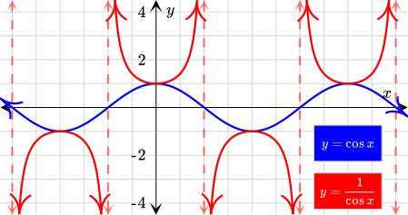
Exploring the Graphs of the Cosine Function and its Reciprocal Function
Discussion
The Secant Function
Let P be the point of intersection of the terminal side of an angle in standard position and the unit circle. The secant function, denoted as sec, is defined as the reciprocal of the x-coordinate of P.
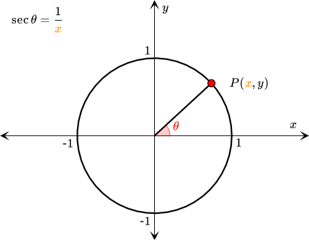
secθ=cosθ1
Since division by 0 is not defined, the graph of the parent secant function y=secx has vertical asymptotes where cosx=0. This means that the graph has vertical asymptotes at odd multiples of x=2π. The graph of y=secx can be drawn by making a table of values.
![The secant function y=sec(x) with asymptotes at -3pi/2, -pi/2, pi/2, 3p/2, and 5pi/2 over the domain [-3pi/2,5pi/2]](/mediawiki/images/7/7a/Mljsx_Concept_Secant_Function_2.svg)
Consider the general form of a secant function.
y=asecbx
Here, a and b are non-zero real numbers and x is measured in radians. The properties of the secant function are be stated in the table below.
| Properties of y=asecbx | |
|---|---|
| Amplitude | No amplitude |
| Number of Cycles in [0,2π] | ∣b∣ |
| Period | ∣b∣2π |
| Domain | All real numbers except odd multiples of 2∣b∣π |
| Range | (-∞,-∣a∣]∪[∣a∣,∞) |
Method
Graphing a Secant Function
Recall the format of a secant function.

The points from the table are (-2π,2.83), (2π,2.83), (23π,-2.83), and (25π,-2.83).
y=asecbθ
Here, a and b are non-zero real numbers and θ is measured in radians. The values of a and b can be used to graph the function. Consider an example function.
y=2sec21θ
In this function, a=2 and b=21. The asymptotes, some points, and the graph of the cosine function can be used to sketch one cycle of a secant curve. Then the cycle can be replicated as many times as desired. Five steps will be followed.
1
Find the Period
expand_more The period of a secant function is the quotient of 2π and ∣b∣.
Period∣b∣2π⇒∣∣∣21∣∣∣2π=4π
The period of this function is 4π. 2
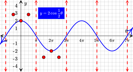
Graph the Related Cosine Function
expand_more Consider the related cosine function.
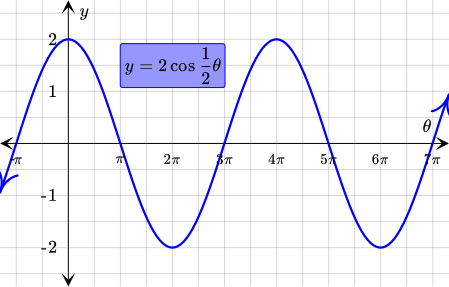
SecantFunctiony=2sec21θRelated CosineFunctiony=2cos21θ
The graph of the cosine function can be drawn on a coordinate plane. 3
Graph the Asymptotes and Plot Points
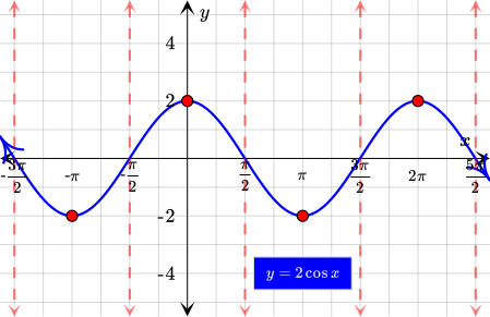
expand_more By definition, the asymptotes of the secant function occur when the output of the cosine function is 0. Furthermore, the maximum and minimum points of the cosine function are also points on the secant function's graph.
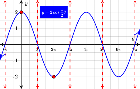
4
Divide the Period and Locate Points
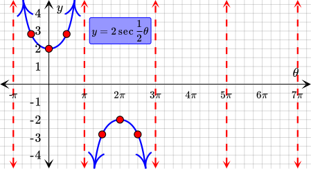
expand_more Here, the period is 4π and the asymptotes occur every 2π radians. Therefore, the asymptotes are located not only at the beginning and at the end of each period, but also in the middle of each period. Divide the interval between two asymptotes in fourths by the following pattern.
Notice that the middle point in the pattern, the maximum or minimum point, was already plotted in the previous step. The remaining four points can be found for the interval that goes from -π to 3π by making a table of values.
| θ | 2sec21θ | y |
|---|---|---|
| -2π | 2sec(21(-2π)) | 22≈2.83 |
| 2π | 2sec(21⋅2π) | 22≈2.83 |
| 23π | 2sec(21⋅23π) | -22≈-2.83 |
| 25π | 2sec(21⋅25π) | -22≈-2.83 |
5
Draw the Graph
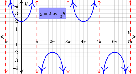
expand_more Finally, the points can be connected with a smooth curve to draw the graph for one cycle.
Once the graph for one cycle is drawn, it can be replicated as many times as desired to draw more cycles. Here, one more cycle will be graphed.
Example
A Bowl and a Secant Function
Ramsha is thinking about a sustainable way of fertilizing her new garden. She collects her kitchen scraps in a bowl so that she can compost them and use the compost for the Tanabata garden. While mixing these scraps with soil to make some fertilizer, Ramsha noticed that the shape of the bowl matches the shape of one branch of a secant function.
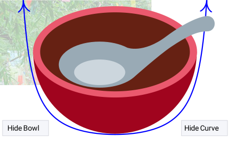 After doing some calculations, she found the equation of the curve that models the bowl.
External credits: Kumiko
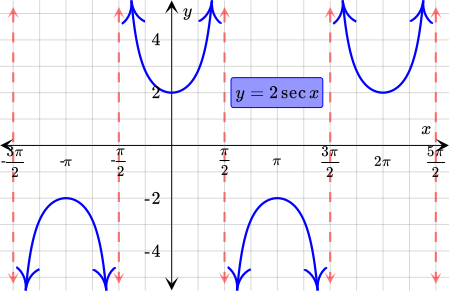
y=2secx
Draw the graph of the above function for values of x between -23π and 25π.
Answer
Hint
Graph the related cosine function and recall that the asymptotes of the secant function occur at the zeros of the cosine function.
Solution
To graph a secant function, the first step is to calculate the period. Consider the general form of a secant function and the given function.
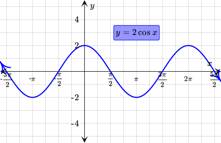 The asymptotes of the secant function occur at the zeros of the cosine function. Furthermore, the maximum and minimum points of the cosine function are also points on the curve of the secant function.
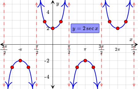
 Next, more points on the curve of y=2secx can be found by making a table of values.
General Formy=asecbxGiven Functiony=2secx⇔y=2sec1x
Here, a=2 and b=1. The period of the function is the quotient of 2π and ∣b∣.
Period∣b∣2π⇒∣1∣2π=2π
Now that it is known that the period of the function is 2π, consider the related cosine function.
SecantFunctiony=2secxRelated CosineFunctiony=2cosx
This cosine function will now be graphed on a coordinate plane for values of x between -23π and 25π. | x | 2secx | y |
|---|---|---|
| -45π | 2sec(-45π) | -22≈-2.83 |
| -43π | 2sec(-43π) | -22≈-2.83 |
| -4π | 2sec(-4π) | 22≈2.83 |
| 4π | 2sec4π | 22≈2.83 |
| 43π | 2sec43π | -22≈-2.83 |
| 45π | 2sec45π | -22≈-2.83 |
| 47π | 2sec47π | 22≈2.83 |
| 49π | 2sec49π | 22≈2.83 |
The points found in the table can now be plotted. Finally, each set of points can be connected with smooth curves.
The graph of the curve of the bowl has been drawn.
Explore
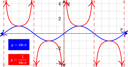
Exploring the Graphs of the Sine Function and its Reciprocal Function
Discussion
The Cosecant Function
Let P be the point of intersection of the terminal side of an angle in standard position and the unit circle. The cosecant function, denoted as csc, is defined as the reciprocal of the y-coordinate of P.
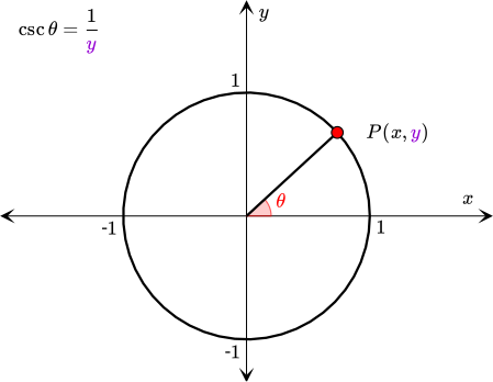
cscθ=sinθ1
Since division by 0 is not defined, the graph of the parent cosecant function y=cscx has vertical asymptotes where sinx=0. This means that the graph has vertical asymptotes at multiples of π. The graph of y=cscx can be drawn by making a table of values.
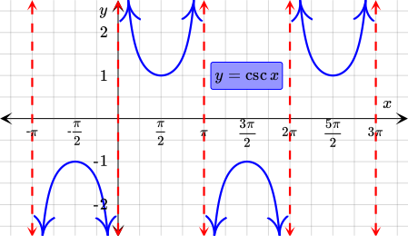
Consider the general form of a cosecant function.
y=acscbx
Here, a and b are non-zero real numbers and x is measured in radians. The properties of the cosecant function are stated below.
| Properties of y=acscbx | |
|---|---|
| Amplitude | No amplitude |
| Number of Cycles in [0,2π] | ∣b∣ |
| Period | ∣b∣2π |
| Domain | All real numbers except multiples of ∣b∣π |
| Range | (-∞,-∣a∣]∪[∣a∣,∞) |
Method
Graphing a Cosecant Function
Recall the format of a cosecant function.

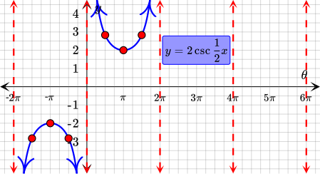
The points found in the table are (-23π,-2.83), (-2π,-2.83), (2π,2.83), and (23π,2.83).

y=acscbθ
Here, a and b are non-zero real numbers and θ is measured in radians. The values of a and b can be used to graph the function. Consider an example function.
y=2csc21θ
In this function, a=2 and b=21. To sketch one cycle of a cosecant curve, its asymptotes, some points, and the graph of the sine function can be used. Then, the cycle can be replicated as many times as desired. Five steps will be followed.
1
Find the Period
expand_more The period of a cosecant function is the quotient of 2π and ∣b∣.
Period∣b∣2π⇒∣∣∣21∣∣∣2π=4π
The period of this function is 4π. 2
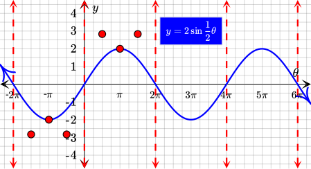
Graph the Related Sine Function
expand_more Consider the related sine function.
![The graph of the sine function 2*sin(1/2 theta) over the domain [-pi,7pi]](/mediawiki/images/3/3e/Mljsx_Method_Graphing_a_Cosecant_Function_1.svg)
CosecantFunctiony=2csc21θRelated SineFunctiony=2sin21θ
The graph of the sine function can be drawn on a coordinate plane. 3
Graph the Asymptotes and Plot Points
expand_more By definition, the asymptotes of the cosecant function occur when the output of the sine function is 0. Furthermore, the maximum and minimum points of the sine function are also points on the cosecant function's graph.
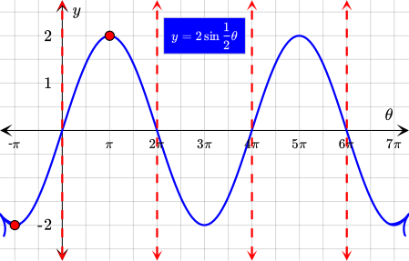
4
Divide the Period and Locate Points
expand_more Here, the period is 4π and the asymptotes occur every 2π radians. Therefore, the asymptotes are located not only at the beginning and at the end of each period, but also in the middle of each period. Divide the interval between two asymptotes in fourths by the following pattern.
Notice that the middle point, which is the maximum or minimum point, was already plotted in the previous step. Four more points can be found for the interval that goes from -2π to 2π by making a table of values.
| θ | 2csc21θ | y |
|---|---|---|
| -23π | 2csc(21(-23π)) | -22≈-2.83 |
| -2π | 2csc(21(-2π)) | -22≈-2.83 |
| 2π | 2csc(21⋅2π) | 22≈2.83 |
| 23π | 2csc(21⋅23π) | 22≈2.83 |
5
Draw the Graph
expand_more Finally, each set of points can be connected with a smooth curve to draw the graph for one cycle.
Once the graph for one cycle is drawn, it can be replicated as many times as desired to draw more cycles. Another cycle is graphed below.
Example
An Umbrella and a Cosecant Function
To protect her new garden, Ramsha decides to set up an umbrella to cover the small plants when heavy rains are forecast. She realizes that the umbrella has the shape of one branch of a cosecant function.
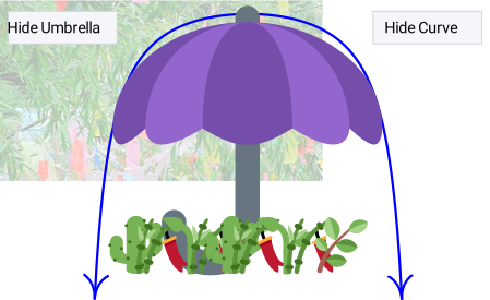 After doing some calculations, she found the equation of the curve that models the umbrella.
External credits: Kumiko
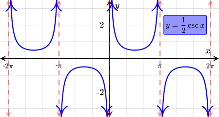
y=21cscx
Draw the graph of the function for values of x between -2π and 2π.
Answer
Hint
Graph the related sine function and recall that the asymptotes of the cosecant function occur at the zeros of the sine function.
Solution
To graph a cosecant function, the first step is to calculate the period. Consider the general form of a cosecant function and the given function.
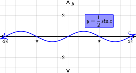 The asymptotes of the cosecant function occur at the zeros of the sine function. Furthermore, the maximum and minimum points of the sine function are also points on the curve of the cosecant function.
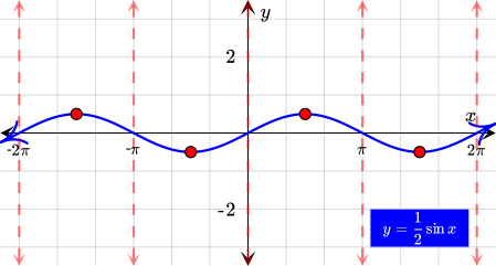 Next, more points on the curve of y=21cscx will be found by making a table of values.
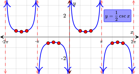
General Formy=acscbxGiven Functiony=21cscx⇔y=21csc1x
Here, a=21 and b=1. The period of the function is the quotient of 2π and ∣b∣.
Period∣b∣2π⇒∣1∣2π=2π
The period of the function is 2π. Now consider the related sine function.
CosecantFunctiony=21cscxRelated SineFunctiony=21sinx
This sine function will now be graphed on a coordinate plane for values of x between -2π and 2π. | x | 21cscx | y |
|---|---|---|
| -35π | 21csc(-35π) | 33≈0.58 |
| -34π | 21csc(-34π) | 33≈0.58 |
| -32π | 21csc(-32π) | -33≈-0.58 |
| -3π | 21csc(-3π) | -33≈-0.58 |
| 3π | 21csc3π | 33≈0.58 |
| 32π | 21csc32π | 33≈0.58 |
| 34π | 21csc34π | -33≈-0.58 |
| 35π | 21csc35π | -33≈-0.58 |
The points found in the table can now be plotted. Finally, connect the sets of points with smooth curves.
Pop Quiz
Finding the Period
Find the period of the following functions. Round the answers to two decimal places.

Closure
Drawing and Using the Graph of a Cosecant Function
The challenge presented at the beginning can be solved with the topics covered in this lesson. It was given that a massive communication tower is anchored to the ground with wires.

y=5cscθ
Here, θ is the measure of the angle formed by the wire and the ground. Graph the function to find the length of the wire that makes an angle of 4π radians with the ground. Round the answer to the nearest integer. {"type":"text","form":{"type":"math","options":{"comparison":"1","nofractofloat":false,"keypad":{"simple":true,"useShortLog":false,"variables":[],"constants":[]},"rendered":false},"text":"<span class=\"katex\"><span class=\"katex-html\" aria-hidden=\"true\"><\/span><\/span>"},"formTextBefore":null,"formTextAfter":"meters","answer":{"text":["7"]}}
Hint
Graph the cosecant function and pay close attention to the y-value for θ=4π.
Solution
To find the length of the wire that makes an angle of 4π radians with the ground, graph the cosecant function. The first step is to calculate the period of the function. Consider the general form of a cosecant function and the given function.
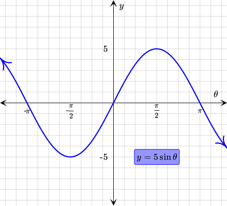 The asymptotes of the cosecant function occur at the zeros of the sine function. Furthermore, the maximum and minimum points of the sine function are also points on the curve of the cosecant function.
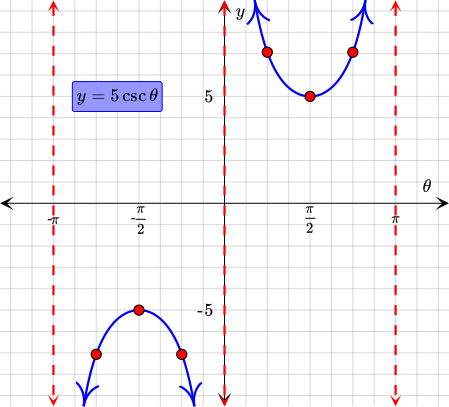
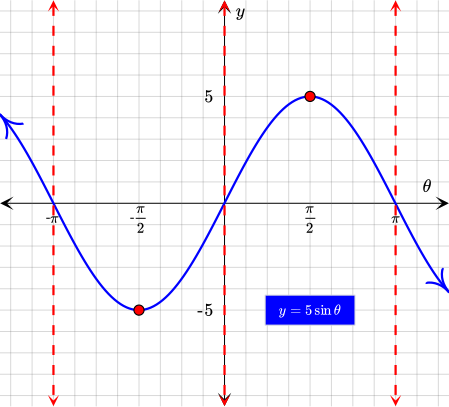 Next, more points on the curve of y=5cscθ will be found by making a table of values.
General Formy=acscbθGiven Functiony=5cscθ⇔y=5csc1θ
Here, a=5 and b=1. The period of the function is the quotient of 2π and ∣b∣.
Period∣b∣2π⇒∣1∣2π=2π
The period of the function is 2π. Now consider the related sine function.
CosecantFunctiony=5cscθRelated SineFunctiony=5sinθ
This sine function can be graphed on a coordinate plane. | θ | 5cscθ | y |
|---|---|---|
| -43π | 5csc(-43π) | -52≈-7.07 |
| -4π | 5csc(-4π) | -52≈-7.07 |
| 4π | 5csc4π | 52≈7.07 |
| 43π | 5csc43π | 52≈7.07 |
Finally, the points found in the table are be plotted and each set of points connected with smooth curves.
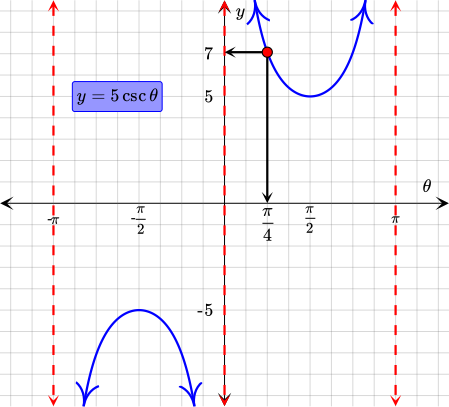
Now that the function has been graphed, the point at θ=4π can be located and its y-coordinate identified.
The exact y-coordinate cannot be found in the graph, but its nearest integer can be identified as 7. Therefore, the length of the wire that makes an angle of 4π radians with the ground is about 7 meters.
Loading content