2. Interpreting Graphs of Linear Equations
Sign In
An error ocurred, try again later!
Chapter 2
2.
Interpreting Graphs of Linear Equations
Linear equations and their graphical representations are fundamental in understanding the relationship between two variables. The concept of the rate of change is pivotal in this understanding. It quantifies how one variable changes in relation to another, providing insights into the behavior of quantities. For instance, the rate of change can be interpreted as speed in certain contexts, such as a car's movement. In the realm of linear equations, every pair of points on a line has a constant rate of change. This consistency is what defines the linearity of the relationship. Furthermore, the slope of a line represents this constant rate of change, making it a crucial element in the study of linear equations. By analyzing graphs, one can derive meaningful interpretations about real-world scenarios, such as a car's speed over time or a student's performance in exams. In essence, the art of interpreting graphs and understanding linear relations is a gateway to making informed predictions and decisions based on data.
Show less Show more expand_more Lesson Settings & Tools
| | 17 Theory slides |
| | 9 Exercises - Grade E - A |
| | Each lesson is meant to take 1-2 classroom sessions |
Interpreting Graphs of Linear Equations
Slide of 17
This lesson will introduce a way to compare and quantify how fast one quantity changes with respect to another. This will allow a more in-depth study of the relationship between two variables and the classification of those variables according to their type of dependency. The ideas covered in this lesson are the foundation of many areas of modern mathematics.
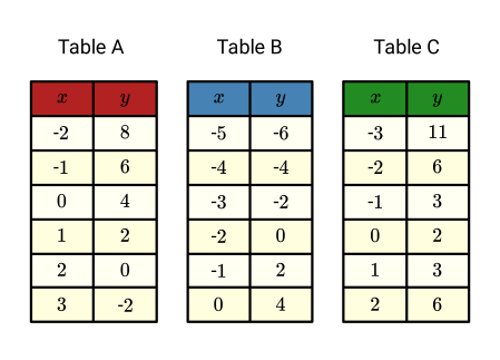 Which of the tables represents the linear equation in two variables y=2x+4?
Catch-Up and Review
Here are a few recommended readings before getting started with this lesson.
- Variables
- Table of Values
- Linear Equations in Two Variables
- Solution of an Equation
- Coordinate Pair
- Coordinate Plane
- Line
Here are a few practice exercises before getting started with this lesson.
a Which of the following equations is a linear equation in two variables?
{"type":"choice","form":{"alts":["x^2+y=25","y=sqrt(x)","y=2x+3","yx= 30"],"noSort":false},"formTextBefore":"","formTextAfter":"","answer":2}
b Consider the linear equation in two variables y=- 3x+5. Which of the following coordinate pairs is a solution to the equation?
{"type":"choice","form":{"alts":["(2,-1)","(0,2)","(3,9)","(0,0)"],"noSort":false},"formTextBefore":"","formTextAfter":"","answer":0}
c Take a look at the tables of values shown below.
{"type":"choice","form":{"alts":["Table A","Table B","Table C"],"noSort":true},"formTextBefore":"","formTextAfter":"","answer":1}
Challenge
Share
Report error
Analyzing Dominika’s Speeds on Her Way to and From School
Dominika is curious about the amount of time she spends going to and from school. One day, she decides to measure the time it takes her to get to school on foot and compare it to the amount of time it takes her to arrive home by bus. She drew the following graph for her trip to school.
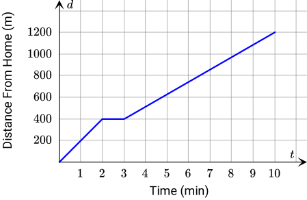
a What was Dominika's average walking speed on the way to school?
b At 2:00PM, the school day was over and Dominika was waiting for the bus. After 9 minutes, the bus finally arrived, and she arrived back home at 2:12PM. Draw a graph similar to the one given in Part A, showing the distance from the school this time, and find Dominika's average speed when returning home.
c Was Dominika faster than the school bus? Explain.
Discussion
Share
Report error
What Is a Rate of Change?
In order to understand the relationship between two quantities and make predictions about their behavior, it is important to be able to compare and quantify how one changes with respect to the other. These ideas define the concept of rate of change.
Concept
Share
Report error
Rate of Change
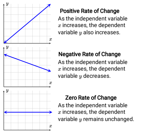
The rate of change ROC is a ratio used to compare how a variable changes in relation to another variable. It is determined by dividing the change in the output variable y by the change in the input variable x. For any ordered pairs (x_1,y_1) and (x_2,y_2), the rate of change is calculated using the following formula.
Rate of Change&= Change in y/Change inx [1em] Rate of Change&= y_2-y_1/x_2-x_1
The Greek letter Δ (Delta) is commonly used to represent a difference. This leads to an alternative way of writing the formula for ROC.
Rate of Change = Δ y/Δ x
Extra
Rate of Change UnitsThe units of a rate of change are the ratio of output units to the input units, meaning that they are derived units. Interpreting the rate of change depends on the context.
| Output Units | Input Units | Rate of Change Units | Possible Interpretation |
|---|---|---|---|
| meters | seconds | meters/second | Car speed over a certain period of time |
| bacteria | hours | bacteria/hour | Growth rate of bacteria in an experiment |
| U.S. dollars | hours | U.S. dollars/hour | Worker's hourly wage |
As mentioned above, the rate of change is a quantity that compares the change in the output variable to the input variable. These are also known as the dependent and independent variables, respectively.
Concept
Share
Report error
Independent and Dependent Variables
In the context of functions, the input is often referred to as the independent variable because it can be chosen arbitrarily from the domain. Conversely, the output is called the dependent variable because its value depends on the value of the independent variable. For instance, if the price of oranges is $ 2.50 per pound, the total cost is determined by the product of the unit price and the weight in pounds. ccccc Cost & & Unit Price & & Weight [0.4em] y & = & 2.50 & * & x
As shown, the total cost of oranges depends on how many pounds of fruit are purchased. Therefore, the cost of oranges y is the dependent variable and the number of pounds purchased x is the independent variable.Example
Share
Report error
Exploring the Rate of Change in Different Scenarios
Diego is taking the bus back to his hometown. During the trip, he sees that there are signs by the side of the road that indicate the distance from the city.
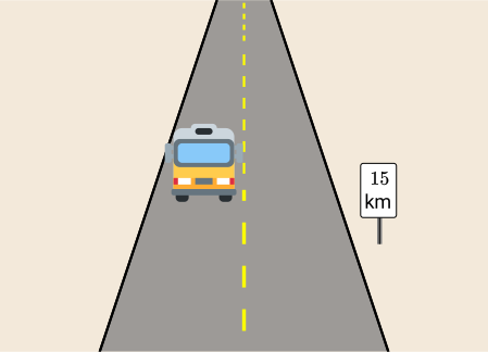
He keeps track of some of the signs and notes the time taken to reach them. He puts the information together using a table of values.
| Time (minutes) | Distance (kilometers) |
|---|---|
| 0 | 0 |
| 10 | 15 |
| 20 | 30 |
| 30 | 45 |
| 40 | 60 |
| 50 | 75 |
| 60 | 90 |
a Considering the variables used in this context, what is the interpretation of the rate of change?
{"type":"choice","form":{"alts":["Speed of the bus","Time taken to reach the destination","Distance covered per liter of gas","Battery performance"],"noSort":false},"formTextBefore":"","formTextAfter":"","answer":0}
{"type":"text","form":{"type":"math","options":{"comparison":"1","nofractofloat":false,"keypad":{"simple":true,"useShortLog":false,"variables":["x"],"constants":["PI"]},"rendered":false},"text":" "},"formTextBefore":null,"formTextAfter":"kmmin","answer":{"text":["1.5"]}}
{"type":"text","form":{"type":"math","options":{"comparison":"1","nofractofloat":false,"keypad":{"simple":true,"useShortLog":false,"variables":["x"],"constants":["PI"]},"rendered":false},"text":" "},"formTextBefore":null,"formTextAfter":"kmmin","answer":{"text":["1.5"]}}
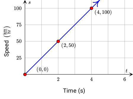
b When he arrived at his hometown, Diego found a magazine containing statistics for different cars. The following graph shows information about the performance of a new electric car, indicating the speed reached during the first few seconds of the car accelerating from zero.
{"type":"text","form":{"type":"math","options":{"comparison":"1","nofractofloat":false,"keypad":{"simple":true,"useShortLog":false,"variables":["x"],"constants":["PI"]},"rendered":false},"text":" "},"formTextBefore":null,"formTextAfter":null,"answer":{"text":["25"]}}
{"type":"text","form":{"type":"math","options":{"comparison":"1","nofractofloat":false,"keypad":{"simple":true,"useShortLog":false,"variables":["x"],"constants":["PI"]},"rendered":false},"text":" "},"formTextBefore":null,"formTextAfter":null,"answer":{"text":["25"]}}
c The magazine also included a linear equation in two variables describing the performance of a hybrid car. This time it refers to the amount of kilometers the car can travel depending on the amount of gallons of gas.
{"type":"text","form":{"type":"math","options":{"comparison":"1","nofractofloat":false,"keypad":{"simple":true,"useShortLog":false,"variables":["x"],"constants":["PI"]},"rendered":false},"text":" "},"formTextBefore":null,"formTextAfter":"km\/gal","answer":{"text":["50"]}}
{"type":"text","form":{"type":"math","options":{"comparison":"1","nofractofloat":false,"keypad":{"simple":true,"useShortLog":false,"variables":["x"],"constants":["PI"]},"rendered":false},"text":" "},"formTextBefore":null,"formTextAfter":"km\/gal","answer":{"text":["50"]}}
{"type":"text","form":{"type":"math","options":{"comparison":"1","nofractofloat":false,"keypad":{"simple":true,"useShortLog":false,"variables":["x"],"constants":["PI"]},"rendered":false},"text":" "},"formTextBefore":null,"formTextAfter":"km\/gal","answer":{"text":["50"]}}
Hint
a In this case, the independent variable is the time, which is measured in seconds. On the other hand, the dependent variable is the distance, which is measured in meters.
b In a coordinate pair, the first coordinate represents the value of the independent variable, while the second coordinate represents the value of the dependent variable.
c A linear equation can be represented by a line on the coordinate plane. When the x-coordinate of a point on the line is known, its y-coordinate can be found by substituting the x-value into the equation of the line.
Solution
a First, the units of the rate of change will be determined and interpreted. Then, the rate of change will be calculated for the given interval.
Interpreting the Rate of Change
The rate of change is defined as the ratio of the change in the dependent variable to the change of the independent variable. Rate of Change = Δ y/Δ x Note that the distance covered by the car depends on the time elapsed. On the other hand, time passes by without relation to the the car and can take any non-negative value without restrictions. Therefore, the dependent variable in this case is the distance, and time is independent. Let t represent the time and d the distance. Rate of Change = Δ d/Δ t = d_2-d_1/t_2-t_1 Recall that the unit of the rate of change is the ratio of the unit of the dependent variable to the unit of the independent variable. Rate of Change Units = kilometers/minute Therefore, the unit of the rate of change is kmmin, which quantifies kilometers traveled per minute. The rate of change can be interpreted as the speed of the bus. Interpretation for the Rate of Change [0.1cm] The speed of the car during a specific period of time
Finding the Rate of Change Between Different Times
Now, by using the rate of change formula together with the information from the table, the rate of change of the car between 10 and 20 minutes will be calculated. Notice that the corresponding distances are 15 and 30 kilometers, respectively.Rate of Change = d_2-d_1/t_2-t_1
SubstitutePoints
Substitute ( 10,15) & ( 20,30)
Rate of Change = 30- 15/20- 10
Rate of Change = 1.5
| Rate of Change = d_2-d_1/t_2-t_1 | ||
|---|---|---|
| Times | Substitute | Evaluate |
| 10- 20 min | 30 km- 15 km/20 min- 10 min | 1.5 kmmin |
| 0- 60 min | 90 km- 0 km/60 min- 0 min | 1.5 kmmin |
b Similarly to Part A, the rate of change formula will be used to find the rate of change of the graph. In this case, the variables are the speed s and the time t.
Rate of Change = s_2-s_1/t_2-t_1
SubstitutePoints
Substitute ( 0,0) & ( 2,50)
Rate of Change = 50- 0/2- 0
Rate of Change = 25
| Rate of Change = y_2-y_1/x_2-x_1 | ||
|---|---|---|
| Points | Substitute | Evaluate |
| ( 0, 0),( 2, 50) | 50- 0/2- 0 | 25 |
| ( 2, 50),( 4, 100) | 100- 50/4- 2 | 25 |
c In this case, before using the rate of change formula, the corresponding x- and y-values must first be found. This can be done by substituting the x-value of interest into the linear equation and evaluating the resulting expression on the right-hand side. This will be done for x= 1 first to illustrate the procedure.
| Linear Equation: y = 2x+3 | ||
|---|---|---|
| x | Substitute | Point |
| x = 1 | y &= 50( 1)+30 y &= 80 | ( 1, 80) |
| x = 3 | y &= 50( 3)+30 y &= 180 | ( 3, 180) |
| x = 4 | y &= 50( 4)+30 y &= 230 | ( 4, 230) |
| x = 7 | y &= 50( 7)+30 y &= 380 | ( 7, 380) |
Now that the points are known, all that is left to do is to repeat the same procedure as in Part B. The following table summarizes the results for the pair of points of interest.
| Rate of Change = y_2-y_1/x_2-x_1 | ||
|---|---|---|
| Points | Substitute | Evaluate |
| ( 1, 80),( 3, 180) | 180- 80/3- 1 | 50 |
| ( 4, 230),( 7, 380) | 380- 230/7- 4 | 50 |
| ( 1, 80),( 7, 380) | 380- 80/7- 1 | 50 |
It is interesting to note that the rate of change is the same between all the pairs of points used. This occurred in Parts A and B as well.
Pop Quiz
Share
Report error
Practice Calculating the Rate of Change
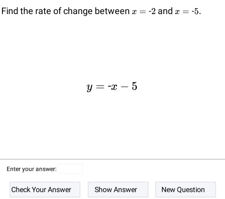
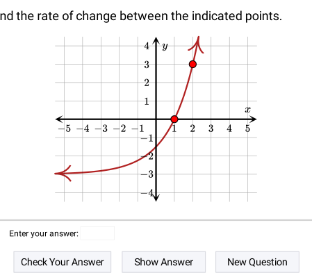
The following applet shows different representations for the data of two variables. Practice finding the rate of change between the indicated values. If the answer is not an integer number, round it to two decimal places.
Discussion
Share
Report error
Linear Relations and Constant Rates of Change
Rule
Share
Report error
Constant Rate of Change
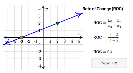
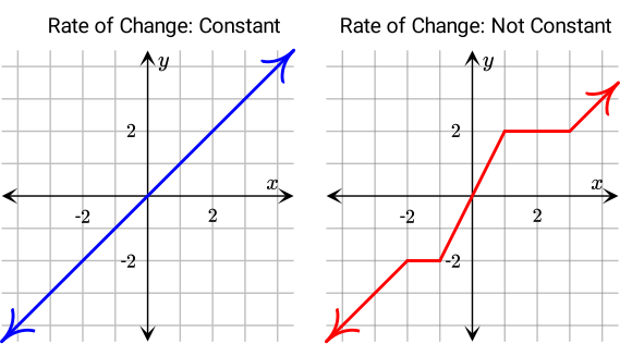
Any line in the coordinate plane has a constant rate of change between any pair of its points. This can be checked by moving the points in the following applet.
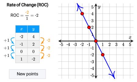
 The opposite of this statement also holds true. If the rate of change between consecutive pairs of points of a data set is constant, then these points follow a linear relation and they all lie on the same line in the coordinate plane. The following applet illustrates this.
Next, it will be shown that every point from the data set satisfies the following linear equation in two variables.
y-y_1 = m (x-x_1)
This will be shown first for the third point from the data set, (x_3,y_3). The expression on the right-hand side of the equation will be rewritten by adding and subtracting y_2 to obtain an identity.
Since (x_3,y_3) and (x_2,y_2), and (x_2,y_2) and (x_1,y_1), are pairs of consecutive points, the differences y_3-y_2 and y_2-y_1 can be rewritten in terms of the constant rate of change m and the corresponding x-values.
Therefore, the third point (x_3,y_3) satisfies the linear equation y-y_1=m(x-x_1). Now it will be shown that the fourth point of the data set, (y_4,x_4), also satisfies the equation.
Recall that it is known that y_4-y_3=m(x_4-x_3) and, from the previous result, it is also known that y_3-y_1 = m (x_3-x_1).
As shown, (x_4,y_4) satisfies the equation as well. This process can be repeated with all the points, and all will satisfy the linear equation y-y_1=m(x-x_1). And since every point satisfies the equation, every point is a solution. Therefore, every point of the data set lies on the line representing this linear equation.
Proof
Algebraic ProofPairs of Points in a Line Have a Constant Rate of Change
Any linear equation in two variables can written in the following form where y is the dependent variable, x is the independent variable, and m and b can be any real numbers. y=mx+b Now, since this is a linear equation in two variables, all of its solutions lie on a line in the coordinate plane. In what follows, two arbitrary points (x_1,y_1) and (x_2,y_2) will be used, and the rate of change between them will be found by using the rate of change formula. Rate of Change = y_2-y_1/x_2-x_1 Because these arbitrary points are solutions to the linear equation, they satisfy the equation. Therefore, it is possible to find an explicit expression for y_1 and y_2 in terms of x_1 and x_2, respectively. y_1 = mx_1+b y_2 = mx_2+b Now that the explicit form for y_1 and y_2 is known, the rate of change between these points can be calculated.Rate of Change = y_2-y_1/x_2-x_1
SubstituteII
y_1= mx_1+b, y_2= mx_2+b
Rate of Change = mx_2+b-( mx_1+b)/x_2-x_1
Rate of Change = m
Consecutive Points in a Data Set with Constant Rate of Change Lie on a Line
Consider a set of data points for which the rate of change between every pair of consecutive points is a constant value m. Consider two consecutive points (x_1,y_1) and (x_2,y_2).
| Rate of Change | Rewrite |
|---|---|
| y_2-y_1/x_2-x_1= m | y_2-y_1 = m (x_2-x_1) |
Note that since the rate of change between every pair of consecutive points is constant, they all can be rewritten in a similar way.
| Rate of Change | Rewrite |
|---|---|
| y_2-y_1/x_2-x_1= m | y_2-y_1 = m (x_2-x_1) |
| y_3-y_2/x_3-x_2= m | y_3-y_2 = m (x_3-x_2) |
| ... | ... |
| y_n-y_(n-1)/x_n-x_(n-1)= m | y_n-y_(n-1) = m (x_n-x_(n-1)) |
y_3-y_1 = y_3-y_2+y_2-y_1
SubstituteII
y_3-y_2= m(x_3-x_2), y_2-y_1= m(x_2-x_1)
y_3-y_1 = m(x_3-x_2)+ m(x_2-x_1)
y_3-y_1 = m (x_3-x_1)
y_4-y_1 = y_4-y_3+y_3-y_1
SubstituteII
y_4-y_3= m (x_4-x_3), y_3-y_1= m (x_3-x_1)
y_4-y_1 = m (x_4-x_3) + m (x_3-x_1)
y_4-y_1 = m (x_4-x_1)
Example
Share
Report error
Identifying Linear Tendencies in Cryptocurrencies
Diego's brother is very interested in crypotcurrencies and is telling Diego about how their values changed in the first weeks of the last year. One of them is of special interest to him because its graph is a straight line. He tried to print some information to show Diego, but his printer broke before it could print the complete tables of values for the cryptocurrencies.
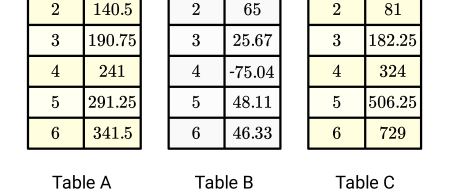
{"type":"choice","form":{"alts":["Table A","Table B","Table C"],"noSort":true},"formTextBefore":"","formTextAfter":"","answer":0}
Hint
Linear relations grow by equal differences over equal intervals.
Solution
In order to identify the data set that follows a linear relation, it is useful to remember that linear relations have a constant rate of change. Therefore, they grow by equal differences over equal intervals. Linear Relation ⇕ Constant Rate of Change Let x represent the week number and y represent the value of the cryptocurrencies. The differences between consecutive x- and y-values will be calculated for each table. This will first be done for Table A.
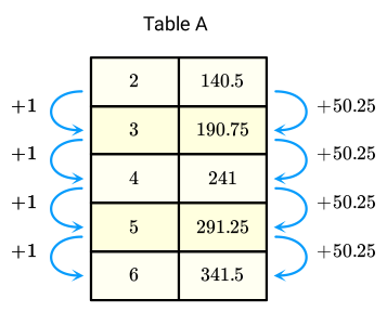
Since the relation represented in Table A increases by equal differences in equal intervals, the data can be modeled with a linear relation. Now, the same procedure will be applied to other tables.
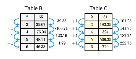
Since the differences between consecutive y-values are not constant for equal intervals, Table B and Table C do not satisfy the condition. As such, they do not represent linear relations.
Pop Quiz
Share
Report error
Identifying Linear Relations From Tables of Values
The following table shows the relationship between two variables, x and y. Look at the data carefully and determine whether the relationship between x and y can be described by linear equation.
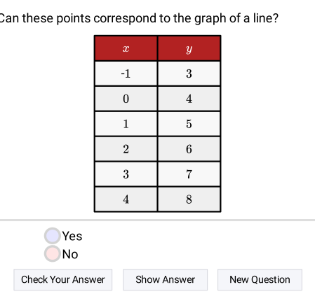
Discussion
Share
Report error
Linear Functions and Intercepts
In a previous example, it was shown how substituting a specific x-value into a linear equation in two variables determined an associated y-value. The set of all the points obtained in this way represent a line in the coordinate plane. This idea is depicted below by showing some points for a particular linear equation.
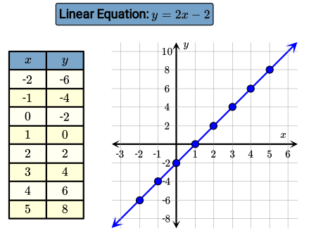
This type of relation in which an input is assigned only one specific output is known as a function. To each input, typically represented by the independent variable x, the function assigns an output represented as f(x). In the example above y depends on x. This can be denoted explicitly by using function notation. ccc Equation & & Function y=2x+1 & & f(x)=2x+1 In general, functions can assign an output value to the input value in many different ways and their graphs can be very different. A particular function whose graph is a line is known as a linear function. Therefore, a linear equation can represent a linear function.
Concept
Share
Report error
Linear Function
A linear function is a function with a constant rate of change. A linear function can be represented by a linear equation in two variables. Graphically, a linear function is a nonvertical line.
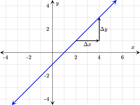
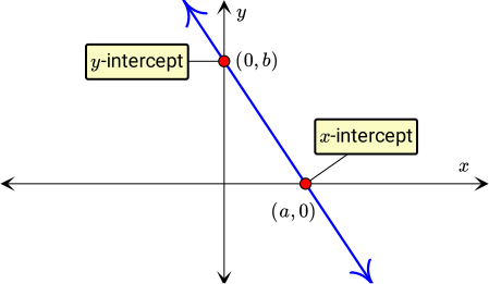
When working with linear functions, there are two points of special interest. These are the points where the line crosses the axes, known as intercepts.
Concept
Share
Report error
Intercept
The x-intercept of a line is the x-coordinate of the point where the line crosses the x-axis. The y-intercept of a line is the y-coordinate of the point where the line crosses the y-axis. The y-intercept of an equation is also known as its initial value.
Example
Share
Report error
Interpreting and Finding the Intercepts of a Linear Function in Different Scenarios
Diego wants to make sure he has enough data available on his smartphone to stream a series while taking a trip with his family. He visits a local branch of his service provider and updates to the Unlimited Plan,
which costs an initial service fee and a special price per gigabyte of data used. The graph represents the costs of the service plan.
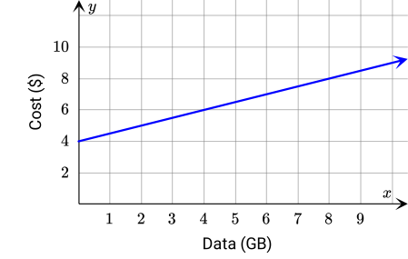
a What is the y-intercept of this linear function? Write the answer as a single number.
{"type":"text","form":{"type":"math","options":{"comparison":"1","nofractofloat":false,"keypad":{"simple":true,"useShortLog":false,"variables":["x"],"constants":["PI"]},"rendered":false},"text":" "},"formTextBefore":null,"formTextAfter":null,"answer":{"text":["4"]}}
{"type":"choice","form":{"alts":["Initial service fee","Total cost of the service","Amount of data used"],"noSort":false},"formTextBefore":"","formTextAfter":"","answer":0}
b After updating his service plan, Diego does some research online about his smartphone model. He finds the following linear function.
{"type":"text","form":{"type":"math","options":{"comparison":"1","nofractofloat":false,"keypad":{"simple":true,"useShortLog":false,"variables":["x"],"constants":["PI"]},"rendered":false},"text":" "},"formTextBefore":null,"formTextAfter":null,"answer":{"text":["10"]}}
{"type":"choice","form":{"alts":["Time it takes for the battery to drain completely","Initial battery charge of the smartphone","Percentage of battery charge used per hour"],"noSort":false},"formTextBefore":"","formTextAfter":"","answer":0}
Hint
a The y-intercept is the y-value corresponding to x=0.
b The x-intercept is the x-value corresponding to y=0.
Solution
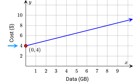
Therefore, the y-intercept is 4. Since this is the cost of the service when 0 gigabytes of data are used, x=0, it can be concluded that $4 is the initial service fee.
b In this case it is necessary to find the x-intercept of the given function. This is the x-value corresponding to y=0. Therefore, to find the x-intercept, y=0 will be substituted into the linear equation and the equation will be solved for x.
y =- 10x +100
Substitute
y= 0
0 =- 10x +100
▼
Solve for x
SubEqn
LHS-100=RHS-100
-100 =- 10x
DivEqn
.LHS /(-10).=.RHS /(-10).
10 = x
RearrangeEqn
Rearrange equation
x =10
Pop Quiz
Share
Report error
Practice Identifying the Intercepts
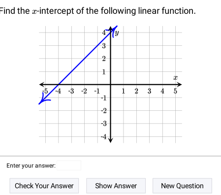
The following applet alternates between a graph and a linear equation, both of which represent linear functions. Identify the indicated intercept of the given function and write the answer as a single number.
Discussion
Share
Report error
Average Rate of Change
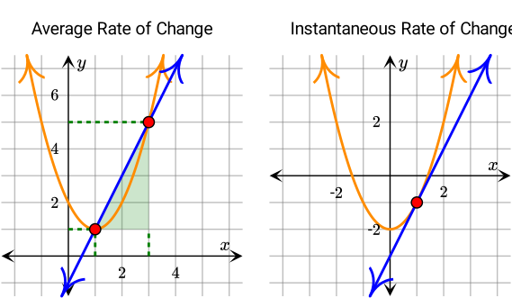
The rate of change of a nonlinear function is not constant — it may even change from point to point. To measure the change for this type of function, an average rate of change is defined by averaging the total change of the function over a specific interval. The following graph illustrates how the average rate of change depends on the interval considered.
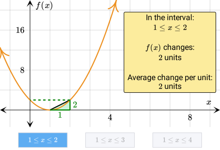 The average rate of change can be thought of as an approximation for the rate of change of the nonlinear function. This approximation is done using the slope of a linear function passing through the endpoints of a specific interval.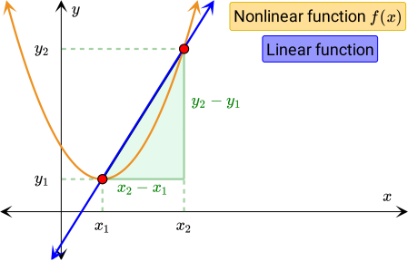
The slope of the linear function can be calculated by using the points common to both functions, (x_1,y_1) and (x_2,y_2). slope = y_2-y_1/x_2-x_1 The y-values that correspond to x_1 and x_2 are also the nonlinear function's values f(x_1) and f(x_2), respectively. Then, the slope formula can be rewritten and identified as the average rate of change of the function f(x) over the interval [x_1, x_2].
Average Rate of Change = f(x_2)-f(x_1)/x_2-x_1Example
Share
Report error
Modeling the Takeoff and Landing Speeds of an Airplane Using Average Rates of Change
Diego decides to fly back home after visiting his family in his hometown. He is very excited as the airplane readies for takeoff. The plane gets into position at the beginning of a long, straight runaway surface and starts accelerating. Diego enjoys the view through the window.

According to this table, which of the following options best approximates the speed of the plane at takeoff?
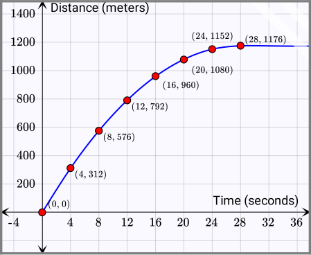 What is the average speed during the first 28 seconds of the landing?
 What is the average speed during the time interval t=24 seconds to t=28 seconds? 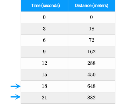 By doing this, the calculation will not average the takeoff speed with the speeds at the beginning and the middle of the motion, and a better approximation for the speed at time of takeoff alone will be obtained. As indicated by the arrows on the table above, the coordinate pairs to be used are (18,648) and (21,882).
It was found that in the interval of time just before takeoff, the average speed of the plane was 78 ms.
The average speed during the first 28 seconds of the landing process is 42 ms. The average speed during the smaller interval, t=24 seconds to t=28 seconds, can be found in the same way.
During this period, the average speed of the plane was just 6 ms, as this calculation included only a short period of time closer to when the plane stopped moving. It does not include the data corresponding to times when the plane had a greater speed, as the average speed for the first 28 seconds of the landing process does.
By doing this, the calculation will not average the takeoff speed with the speeds at the beginning and the middle of the motion, and a better approximation for the speed at time of takeoff alone will be obtained. As indicated by the arrows on the table above, the coordinate pairs to be used are (18,648) and (21,882).
It was found that in the interval of time just before takeoff, the average speed of the plane was 78 ms.
The average speed during the first 28 seconds of the landing process is 42 ms. The average speed during the smaller interval, t=24 seconds to t=28 seconds, can be found in the same way.
During this period, the average speed of the plane was just 6 ms, as this calculation included only a short period of time closer to when the plane stopped moving. It does not include the data corresponding to times when the plane had a greater speed, as the average speed for the first 28 seconds of the landing process does.
a On the screen in front of his seat, Diego can see statistics of the flight in progress. He selects the option to display the information about the takeoff as a table of values, which shows the distance covered by the airplane at a specific time period during the takeoff process. He obtains the following information.
| Time (seconds) | Distance (meters) |
|---|---|
| 0 | 0 |
| 3 | 18 |
| 6 | 72 |
| 9 | 162 |
| 12 | 288 |
| 15 | 450 |
| 18 | 648 |
| 21 | 882 |
{"type":"choice","form":{"alts":["48 ms","66 ms","78 ms","90 ms"],"noSort":false},"formTextBefore":"","formTextAfter":"","answer":2}
b The trip has been completed and the plane is finally landing. Diego is curious about the statistics for the landing process. This time he chooses to display the data using a graph. The graph shows the distance covered after the airplane came in contact with the runaway and started decelerating.
{"type":"text","form":{"type":"math","options":{"comparison":"1","nofractofloat":false,"keypad":{"simple":false,"useShortLog":false,"variables":["x"],"constants":["PI"]},"rendered":false},"text":" "},"formTextBefore":null,"formTextAfter":"ms","answer":{"text":["42"]}}
{"type":"text","form":{"type":"math","options":{"comparison":"1","nofractofloat":false,"keypad":{"simple":false,"useShortLog":false,"variables":["x"],"constants":["PI"]},"rendered":false},"text":" "},"formTextBefore":null,"formTextAfter":"ms","answer":{"text":["6"]}}
Hint
a The rate of change represents the speed of the plane, which is not constant. Therefore, the takeoff speed can be approximated by averaging over an interval as specific to the takeoff as possible.
b Identify the intervals of interest and use the formula for the average rate of change.
Solution
a In this case, the rate of change represents the speed of the plane. Since the plane is accelerating, its speed is increasing and the rate of change from the table of values is not constant. Then, the best that can be done is to approximate the speed by using the average rate of change formula.
Average Rate of Change = d_2-d_1/t_2-t_1 Note that since distance covered depends on the time value but time has no restriction, distance d is the dependent variable and time t is the independent variable. Now, to best approximate the speed at takeoff, the interval used for finding the average rate of change should be as short and as close to takeoff as possible.
Average Rate of Change = d_2-d_1/d_2-d_1
SubstitutePoints
Substitute ( 18,648) & ( 21,882)
Average Rate of Change = 882- 648/21- 18
Average Rate of Change = 78
b For this exercise, the average speed during the first 28 seconds of the landing process must be found. To find it, the interval to be used is t=0 seconds to t=28 seconds. The average speed can be found by using these values together with their corresponding distances.
Average Rate of Change = d_2-d_1/t_2-t_1
SubstitutePoints
Substitute ( 0,0) & ( 28,1176)
Average Rate of Change = 1176- 0/28- 0
Average Rate of Change = 42
Average Rate of Change = d_2-d_1/t_2-t_1
SubstitutePoints
Substitute ( 24,1152) & ( 28,1176)
Average Rate of Change = 1176- 1152/28- 24
Average Rate of Change = 6
Pop Quiz
Share
Report error
Practice Calculating the Average Rate of Change
The following applet shows different representations for the data of two variables. Practice finding the average rate of change between the indicated values. If the answer is not an integer number, round it to two decimal places.
Discussion
Share
Report error
Rate of Change for Graphs Comprised of Different Lines
It is important to mention that the graphs of some functions can be comprised of straight lines with different slopes. The average rate of change is used for these functions as well, since the graph is not a single straight line and the rate of change is not constant.
Example
Share
Report error
Analyzing Dominika’s Speeds on Her Way to and From School
Dominika is curious about the amount of time she spends going to and from school. One day, she decides to measure the time it takes her to get to school on foot and compare it to the amount of time it takes her to arrive home by bus. She drew the following graph for her trip to school.
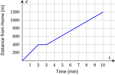
a What was Dominika's average walking speed on the way to school?
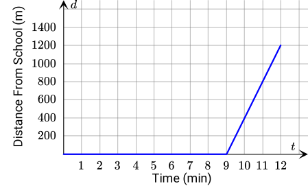
b At 2:00PM, the school day was over and Dominika was waiting for the bus. After 9 minutes, the bus finally arrived, and she arrived back home at 2:12PM. Draw a graph similar to the one given in Part A, showing the distance from the school this time, and find Dominika's average speed when returning home.
c Was Dominika faster than the school bus? Explain.
Answer
a 120 meters per minute
b Graph:
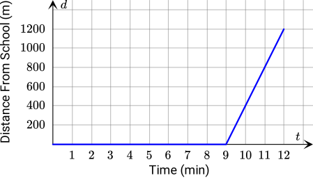
Average Speed: 100 meters per minute
c No, see solution.
Hint
a Use the formula for the average rate of change. Use the information from the graph to identify the appropriate interval to be used in the calculation.
b Use the formula for the average rate of change. Use the information from the graph to identify the appropriate interval to be used in the calculation.
c Think carefully about what is being averaged in Part B.
Solution
a In this case, the dependent variable represents the distance covered in meters, while the independent variable represents the time in minutes required to cover that distance. The units of the rate of change are the ratio of the units of the dependent variable to the units of the independent variable.
Average Rate of Change = d_2-d_1/t_2-t_1
SubstitutePoints
Substitute ( 0,0) & ( 10,1200)
Average Rate of Change = 1200- 0/10- 0
Average Rate of Change = 120
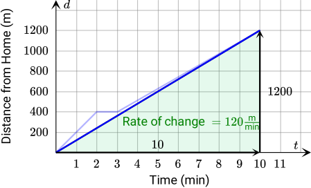
b To draw the graph, remember that Dominika waited for the bus for the first 9 minutes. During this period of time, her position did not change and she was constantly 0 meters away from school.
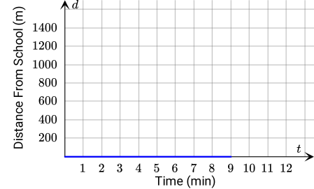
After this time, she got on the bus and arrived back home at t=12 minutes. Recall that the distance between her home and her school is 1200 meters.
Average Rate of Change = d_2-d_1/t_2-t_1
SubstitutePoints
Substitute ( 0,0) & ( 12,1200)
Average Rate of Change = 1200- 0/12- 0
Average Rate of Change = 100
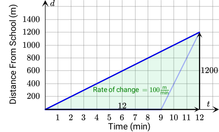
c The fact that Dominika's average speed on her way to school was greater than the average speed when returning home may seem confusing since she went to school on foot and returned by bus. How can this be possible?
Average speed going to school on foot 120 mmin [1.5em] Average speed returning from school by bus 100 mmin
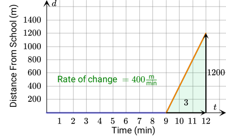
This does not mean that Dominika's average speed was greater than the bus's. For the calculation of the return trip, the 9 minutes that Dominika waited — and therefore did not move — were averaged together with the motion of the bus. The following graph shows the waiting period and the bus ride in different colors.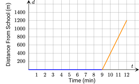
Average Rate of Change = d_2-d_1/t_2-t_1
SubstitutePoints
Substitute ( 9,0) & ( 12,1200)
Average Rate of Change = 1200- 0/12- 9
Average Rate of Change = 400
Closure
Share
Report error
Summary and Further Applications for the Rate of Change
In this lesson, the concepts of x- and y-intercepts, as well as linear functions, were introduced. However, it is important to note that the concept of a function is more general and that there are also nonlinear functions.
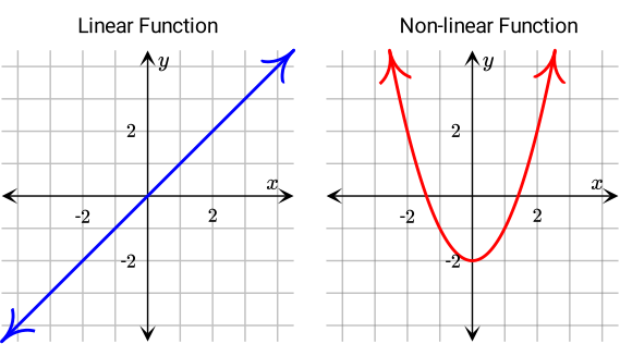
Other main ideas of the lesson were the rate of change and the average rate of change. These basic concepts lead to the definition of instantaneous rate of change. Unlike the average rate of change, which is an approximation for an interval, the instantaneous rate of change gives the exact value of the rate of change at a specific point.
Interpreting Graphs of Linear Equations
The following table models Tadeo's income y, in dollars, for working x hours.
![table; x-column=[4,5,6,7]; y-column=[46.60,A,B,81.55]](/mediawiki/images/d/d0/Mljsx_Exercise_2779_0.svg)
{"type":"text","form":{"type":"math","options":{"comparison":"1","nofractofloat":false,"keypad":{"simple":true,"useShortLog":false,"variables":[],"constants":[]},"rendered":false},"text":" "},"formTextBefore":"B=","formTextAfter":null,"answer":{"text":["69.9"]}}
security
report
code
security
report
code
We want to find the missing values in our table of values. Let's begin by trying to identify a pattern of change between consecutive rows.
We can see that the change in x from one row to the next one is 1, but we cannot determine the change in the y-values for consecutive rows. However, because the values follow a liner relationship, the rate of change is constant. This means that the rate of change between x=4 and x=5 is the same as the rate of change between x=4 and x=7. Rate of change = 81.55-46.60/7-4 Let's solve for the rate of change.
The rate of change is 11.65, which means that the y-values increase by 11.65 between consecutive rows. In context, this means that Tadeo earns $11.65 per hour. His wage is constant, so we can find the value of A by adding 11.65 to 44.60. Then we can increase A by 11.65 again to find the value of B.
We found that A= 58.25 and B= 69.90.
security
report
code
Interpreting Graphs of Linear Equations
Recommended exercises
To get personalized recommended exercises, please login first.
Loading content
≤
>
■2
■▢
e▢
7
8
9
×
÷■1
=
=
√▢
▢√
∫▢▢
4
5
6
+
−
≤
<
log
ln
log▢
1
2
3
()
∣
sin
cos
tan
0
.
π
x
y
Loading content