{{ tocSubheader }}
{{ 'ml-label-loading-course' | message }}
An error ocurred, try again later!
Chapter {{ article.chapter.number }}
{{ article.number }}.
{{ article.displayTitle }}
{{ article.intro.summary }}
Show less Show more expand_more Lesson Settings & Tools
| | {{ 'ml-lesson-number-slides' | message : article.intro.bblockCount }} |
| | {{ 'ml-lesson-number-exercises' | message : article.intro.exerciseCount }} |
| | {{ 'ml-lesson-time-estimation' | message }} |
Analyzing and comparing data is as important as collecting it. This lesson covers basic data analysis concepts. It starts with finding a central value and then moves on to measuring how spread out the data points are. A good understanding of statistical measures will be achieved through this lesson.
Catch-Up and Review
Here is a recommended readings before getting started with this lesson.
Challenge
Study a Data Set About The Lifespan of Cats
Emily and Ignacio love learning about animals. They believe they can make meaningful discoveries by studying data about any animal, beginning with cats. They choose to create a data set, consisting of seven data points, showing the lifespan of cats in their neighborhood. They surveyed their neighbors to get this information.
| Lifespan of Cats (in years) | |||
|---|---|---|---|
| 15 | 11 | 14 | 15 |
| 14 | 17 | 13 | |
Answer the following questions using this data set.
a What is the average lifespan of a cat?
{"type":"text","form":{"type":"math","options":{"comparison":"1","nofractofloat":false,"keypad":{"simple":true,"useShortLog":false,"variables":["x"],"constants":["PI"]},"rendered":false},"text":"<span class=\"katex\"><span class=\"katex-html\" aria-hidden=\"true\"><\/span><\/span>"},"formTextBefore":null,"formTextAfter":"years","answer":{"text":["14.1"]}}
b Which number, if any, occurs most frequently?
{"type":"text","form":{"type":"list","options":{"comparison":"1","nofractofloat":false,"keypad":{"simple":true,"useShortLog":false,"variables":["x"],"constants":["PI"]},"rendered":false,"ordermatters":false,"numinput":2,"listEditable":true,"hideNoSolution":true},"text":"<span class=\"katex\"><span class=\"katex-html\" aria-hidden=\"true\"><\/span><\/span>"},"formTextBefore":null,"formTextAfter":"years","answer":{"text":["14","15"]}}
c Rearrange the data from least to greatest. What number is in the middle of this sorted data set?
{"type":"text","form":{"type":"math","options":{"comparison":"1","nofractofloat":false,"keypad":{"simple":true,"useShortLog":false,"variables":["x"],"constants":["PI"]},"rendered":false},"text":"<span class=\"katex\"><span class=\"katex-html\" aria-hidden=\"true\"><\/span><\/span>"},"formTextBefore":null,"formTextAfter":"years","answer":{"text":["14"]}}
Discussion
What is a Data Set?
A data set is a collection of values that provides information. These values can be presented in various ways such as in numbers or categories. The values are typically gathered through measurements, surveys, or experiments. Consider a data set that consists of the heights of a group of actors.
| Actor | Height |
|---|---|
| Madzia | 5 ft 4 in. |
| Magda | 5 ft 2 in. |
| Ignacio | 6 ft 1.6 in. |
| Henrik | 5 ft 10 in. |
| Ali | 6 ft 1 in. |
| Diego | 5 ft 2 in. |
| Miłosz | 5 ft 2 in. |
| Paulina | 5 ft 3 in. |
| Aybuke | 5 ft 7 in. |
| Mateusz | 6 ft 1.2 in. |
| Gamze | 5 ft 3 in. |
| Marcin | 5 ft 7 in. |
| Marcial | 5 ft 8 in. |
| Heichi | 5 ft 5 in. |
| Arkadiusz | 5 ft 6 in. |
| Enrique | 5 ft 10.5 in. |
| Aleksandra | 5 ft 4 in. |
| Ashli | 5 ft 4 in. |
| Jordan | 5 ft 5 in. |
| Paula | 5 ft 2 in. |
| MacKenzie | 5 ft 6 in. |
| Joe | 6 ft 1 in. |
| Flavio | 5 ft 10 in. |
| Jeremy | 5 ft 4 in. |
| Umut | 6 ft 1 in. |
Number of Observations: Number of Variables: 242
The actual number or category associated with each data point is called a data value. Data values are the specific pieces of information contained within a data point. Data sets can be represented using charts, tables, or different types of graphs. For example, the average temperature of a city for each month of 2018 can be plotted on a line graph. 
Discussion
What is the Average of a Data Set?
The mean, or the average, of a numerical data set is one of the measures of center. It is defined as the sum of all of the data values in a set divided by the number of values in the set.
Mean=Number of ValuesSum of Values
The following applet calculates the mean of the data set on the number line. Points can be moved to change the data values.

Discussion
What is the Median of a Data Set?
The median is a measure of center that lies in the middle of a numerical data set when the data set is written in numerical order. When the the data set has an odd number of data points, the median is the value in the middle.
 However, when the the data set has an even number of data points, the median is the average of the two middle numbers.
Discussion
What is the Mode of a Data Set?
The mode is a measure of center that shows the most common value in a data set. Modes can be used for both numerical and categorical data.
 A data set can have more than one mode if two or more data values are equally common. However, if all values in the set only occur once, then the data set does not have a mode.
Discussion
Summarizing a Data Set With a Single Number
A measure of center, or a measure of central tendency, is a statistic that summarizes a data set by finding a central value. The most common measures of center are the mean, median, and mode.  Move the points around in the dot plot to generate new data. The applet identifies the mean, median, and mode of the data set.
Example
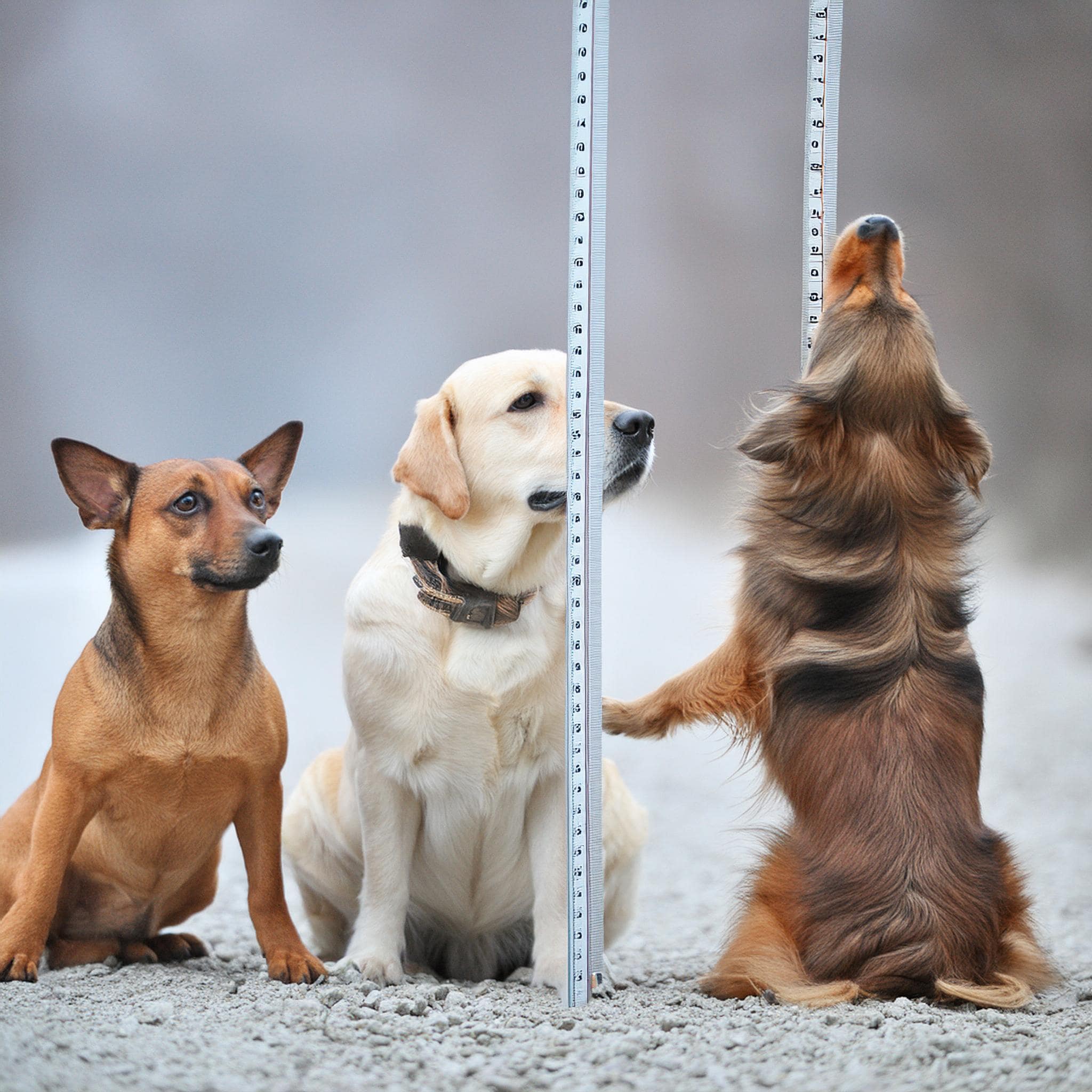
Studying Data about the Lifespan of Dogs
Ignacio volunteers at a dog shelter. He asks Emily to help him study a data set he made concerning the lifespan of some of the dogs. The information they gather will help the shelter!
 This time, the data set consists of eight data points rather than seven.
| Lifespan of Dogs (in years) | |||
|---|---|---|---|
| 10 | 21 | 16 | 15 |
| 13 | 15 | 17 | 11 |
a What is the mean of the data set?
{"type":"text","form":{"type":"math","options":{"comparison":"1","nofractofloat":false,"keypad":{"simple":true,"useShortLog":false,"variables":["x"],"constants":["PI"]},"rendered":false},"text":"<span class=\"katex\"><span class=\"katex-html\" aria-hidden=\"true\"><\/span><\/span>"},"formTextBefore":null,"formTextAfter":"years","answer":{"text":["14.75"]}}
b What is the median of the data set?
{"type":"text","form":{"type":"math","options":{"comparison":"1","nofractofloat":false,"keypad":{"simple":true,"useShortLog":false,"variables":["x"],"constants":["PI"]},"rendered":false},"text":"<span class=\"katex\"><span class=\"katex-html\" aria-hidden=\"true\"><\/span><\/span>"},"formTextBefore":null,"formTextAfter":"years","answer":{"text":["15"]}}
c What is the mode of the data set?
{"type":"text","form":{"type":"math","options":{"comparison":"1","nofractofloat":false,"keypad":{"simple":true,"useShortLog":false,"variables":["x"],"constants":["PI"]},"rendered":false},"text":"<span class=\"katex\"><span class=\"katex-html\" aria-hidden=\"true\"><\/span><\/span>"},"formTextBefore":null,"formTextAfter":"years","answer":{"text":["15"]}}
Hint
a The mean of the data set is the sum of the data values divided by the number of data values.
b Order the data from least to greatest. What number is in the middle?
c The mode of a data set is the value that occurs most frequently.
Solution
a The mean of a data set is calculated by finding the sum of all values in the set and then dividing by the number of values in the set. In this case, there are 8 values in the set.
10,21,16,15,13,15,17,11
Add all values and divide the sum by 8.
Mean=Number of ValuesSum of Values
SubstituteValues
Substitute values
Mean=810+21+16+15+13+15+17+11
AddTerms
Add terms
Mean=8118
CalcQuot
Calculate quotient
Mean=14.75
b Start by ordering the values from least to greatest.
Unordered Data Set10,21,16,15,13,15,17,11⇓Ordered Data Set10,11,13,15,15,16,17,21
The number of values matters when determining the median. - For a set with an odd number of values, the median is the middle value.
- For a set with an even number of values, the median is the mean of the two middle values.
Ordered Data Set10,11,13,15,15,16,17,21
Therefore, the median of the data set is the mean of 15 and 15.
The median of this data set is 15 years.
c Remember that the mode of a data set is the value or values that occur most often. Take another look at the given data set.
Ordered Data Set10,11,13,15,15,16,17,21
As seen, 15 occurs two times and the rest of the numbers occurs only once. This means that the mode of the data set is 15 years. Note that while the mean, median, and mode are close in this instance, they may vary in other cases.
Pop Quiz
Practice Finding Measures of the Center

Discussion
Measures of Spread of Data Sets
Similar to the measures of center, there are measures that describe how much the values in a data set differ from each other using only one measure. These measures summarize the spread of the data.
Concept
Range
Range is a measure of spread that measures the difference between the maximum and minimum values of the data set.

Discussion
Quartiles
Quartiles are three values that divide a data set into four equal parts. The quartiles are denoted as Q1, Q2, and Q3. The second quartile Q2, also known as the median, divides the ordered data set into two halves. 
Lower halfa b cQ2↑dUpper halfe f g
The median of the lower half is the first quartile Q1, while the median of the upper half is the third quartile Q3. Lower halfa b c↓Q1Q2↑dUpper halfe f g↓Q3
The first quartile is also called lower quartile, and the third quartile is also called upper quartile. To find the quartiles of a data set, the values must first be written in numerical order. Discussion
Interquartile Range
The interquartile range, or IQR, of a data set is a measure of spread that measures the difference between Q3 and Q1, the upper and lower quartiles.
IQR=Q3−Q1
The following applet shows how to find the IQR of different data sets.

Discussion
Finding the Interquartile Range
The interquartile range (IQR) of a data set is found by first identifying the three quartiles and then calculating the difference between the third and the first quartile. Consider the following data set.


1, 3, 4, 4, 5, 6, 6, 8, 8, 10, 10, 11
The interquartile range of the data set can be found by following these four steps.
1
Identify the Median
expand_more First, identify the median of the given data set. Since the number of values is even, the median is the mean of the two middle values.
The median of the data is 6.
2
Identify the Lower and the Upper Half of the Data Set
expand_more The median divides the data into two halves, a lower half and an upper half. For this data, the lower half includes the first six values and the upper half includes the following six.
When there is an odd number of values in the data set, the middle value is excluded from both the lower and upper sets.
3
Find the First and the Third Quartile
expand_more Find the first and the third quartile. The first quartile, Q1, is the median of the lower set, while the third, Q3, is the median of the upper set. Here, both quartiles are found the same way the median was found.
4
Calculate the Interquartile Range
expand_more The interquartile range is calculated by subtracting the first quartile, Q1, from the third, Q3. For the given data set, the first quartile is 4 and the third quartile is 9.
IQR =Q3−Q1=9−4=5
The interquartile range of the given data set is 5. Example
Comparing the Weights of Cats and Dogs
Ignacio and Emily enjoyed learning about cats and dog so much that they now want to compare the spread of one data set with the spread of another.
 They collected a few more data points and compiled a data set consisting of nine data points for the weights of cats.

 The first quartile is 7.5, and the third quartile is 11. The difference between the third quartile and the first quartile is the interquartile range.
The interquartile range of cat weights is 3.5 pounds.
The first quartile is 7.5, and the third quartile is 11. The difference between the third quartile and the first quartile is the interquartile range.
The interquartile range of cat weights is 3.5 pounds. 
 The first quartile is 29, and the third quartile is 44. The difference between the third quartile and the first quartile is the interquartile range.
The interquartile range of dog weights is 15 pounds.
The first quartile is 29, and the third quartile is 44. The difference between the third quartile and the first quartile is the interquartile range.
The interquartile range of dog weights is 15 pounds.
 They collected a few more data points and compiled a data set consisting of nine data points for the weights of cats.
Weights of Cats (lb)9, 8, 11, 7, 10, 7, 11, 8, 12
Then, they collected a data set of ten data points for the weights of dogs.
Weights of Dogs (lb)11, 18, 29, 32, 32, 35, 37, 44, 55, 79
a Which type of pet has a larger weight range: dogs or cats?
{"type":"choice","form":{"alts":["Cats","Dogs","Both have the same weight range"],"noSort":false},"formTextBefore":"","formTextAfter":"","answer":1}
b Find the interquartile range of each data set.
{"type":"text","form":{"type":"math","options":{"comparison":"1","nofractofloat":false,"keypad":{"simple":true,"useShortLog":false,"variables":["x"],"constants":["PI"]},"rendered":false},"text":"<span class=\"katex\"><span class=\"katex-html\" aria-hidden=\"true\"><\/span><\/span>"},"formTextBefore":"Interquartile Range of Cat Weights:","formTextAfter":"lb","answer":{"text":["3.5"]}}
{"type":"text","form":{"type":"math","options":{"comparison":"1","nofractofloat":false,"keypad":{"simple":true,"useShortLog":false,"variables":["x"],"constants":["PI"]},"rendered":false},"text":"<span class=\"katex\"><span class=\"katex-html\" aria-hidden=\"true\"><\/span><\/span>"},"formTextBefore":"Interquartile Range of Dog Weights:","formTextAfter":"lb","answer":{"text":["15"]}}
Hint
a The range of the data set is the difference between the greatest and least data values.
b The interquartile range is the distance between the first and the third quartiles of the data set.
Solution
a The range is one of the measures of spread. It is the difference between the maximum and minimum values of the data set. The range of each data set will be calculated individually.
Range for the Weights of Cats
The least and greatest values can be identified without sorting the data values. Note that they can be listed in order if desired.Weights of Cats (lb)9, 8, 11, 7, 10, 7, 11, 8, 12
The least value is 7 and the greatest value is 12. The difference between these values is 12−7=5.
Range12−7=5 lb
The range for the weights of cats is 5 pounds. Range for the Weights of Dogs
Apply the same procedure of identifying the greatest and least values for the data set of dogs.Weights of Dogs (lb)11, 18, 29, 32, 32, 35, 37, 44, 55, 79
The least value is 11 and the greatest value is 59. The difference between these values is 79−11=68. Range79−11=68 lb
Dogs have a weight range of 68 pounds. This far exceeds the 5-pound range for cats.
b The interquartile range of each data set will be calculated individually.
Interquartile Range of Cat Weights
Here, it is necessary to order the values from least to greatest. Then identify the median of the given data set. Since the number of values is an odd number, the median is the middle value.
The median of the data is 9. Both the lower and upper halves contain four data values. Therefore, there are two middle values in each half. The median of each half is the mean of the two middle values.
Interquartile Range of Dog Weights
In this case, the data values are ordered from least to greatest and the number of values is an even number. This means that the median is the mean of the two middle values.
The median of the data is 33.5. Both the lower and upper halves contain five data values. Therefore, there is only one middle value in each half.
Discussion
Five-Number Summary
A five-number summary of a data set consists of the following five values.
These values provide a summary of the central tendency and spread of the data set. The five-number summary is useful for understanding the variability in a data set. When the data set is written in numerical order, the median divides the data set into two halves. The median of the lower half is the first quartile Q1 and the median of the upper half is the third quartile Q3.

Discussion
Outliers
An outlier is a data point that is significantly different from the other values in the data set. It can be significantly larger or significantly smaller than the others.

Categorical data sometimes also have unusual elements; these can be called outliers as well.

What Does Significantly Different
Mean?
For numerical data, the following definition is one of the several approaches that can be used.
- A data value is an outlier — significantly different from the other values — if it is farther away from the closest quartile than 1.5 times the interquartile range.
Such a value was suggested by the esteemed American mathematician John Tukey. Move the slider in the following applet to see which data point is an outlier.

Example
An Unusual Value in the Data
Ignacio is relaxing, enjoying reviewing some data.  Wait a minute! There is something unusual about a data value in the data set for dogs.
 The interquartile range of this data set is 15. Now calculate Q3+1.5IQR.
This means that any value greater than 66.5 is an outlier. Therefore, the value 79 is an outlier.
The interquartile range of this data set is 15. Now calculate Q3+1.5IQR.
This means that any value greater than 66.5 is an outlier. Therefore, the value 79 is an outlier.

 The first quartile is 23.5, and the third quartile is 40.5. The difference between the third quartile and the first quartile is the interquartile range.
The interquartile range of the data when the outlier is taken out of the data set is 17.
The first quartile is 23.5, and the third quartile is 40.5. The difference between the third quartile and the first quartile is the interquartile range.
The interquartile range of the data when the outlier is taken out of the data set is 17.
 Wait a minute! There is something unusual about a data value in the data set for dogs.
Weights of Dogs (lb)11, 18, 29, 32, 32, 35, 37, 44, 55, 79
a Identify the outlier in the data set.
{"type":"text","form":{"type":"math","options":{"comparison":"1","nofractofloat":false,"keypad":{"simple":true,"useShortLog":false,"variables":["x"],"constants":["PI"]},"rendered":false},"text":"<span class=\"katex\"><span class=\"katex-html\" aria-hidden=\"true\"><\/span><\/span>"},"formTextBefore":null,"formTextAfter":null,"answer":{"text":["79"]}}
b Find the range and interquartile range of the data set without the outlier.
{"type":"text","form":{"type":"math","options":{"comparison":"1","nofractofloat":false,"keypad":{"simple":true,"useShortLog":false,"variables":["x"],"constants":["PI"]},"rendered":false},"text":"<span class=\"katex\"><span class=\"katex-html\" aria-hidden=\"true\"><\/span><\/span>"},"formTextBefore":"Range:","formTextAfter":"lb","answer":{"text":["44"]}}
{"type":"text","form":{"type":"math","options":{"comparison":"1","nofractofloat":false,"keypad":{"simple":true,"useShortLog":false,"variables":["x"],"constants":["PI"]},"rendered":false},"text":"<span class=\"katex\"><span class=\"katex-html\" aria-hidden=\"true\"><\/span><\/span>"},"formTextBefore":"Interquartile Range:","formTextAfter":"lb","answer":{"text":["17"]}}
c Which measure does the outlier affect more?
{"type":"choice","form":{"alts":["Range","Interquartile Range"],"noSort":false},"formTextBefore":"","formTextAfter":"","answer":0}
Hint
a Is there a value that is larger or smaller than most values? Check if there is any value less than Q1−1.5IQR or greater than Q3+1.5IQR.
b The range of a data set is the difference between the greatest and smallest data values. The interquartile range of a data set is the distance between the first and the third quartiles of the data set.
c Compare the range and interquartile range of the data set with and without the outlier.
Solution
a In the given data set, all values seem to be around the same number, except 79. This value seems to be significantly different from other values. Therefore, it is likely to be an outlier of the data set.
Weights of Dogs (lb)11, 18, 29, 32, 32, 35, 37, 44, 55, 79
To confirm that, check if it is farther away from the closest quartile by 1.5 times the interquartile range. The first quartile of this data is 24, and the third quartile is 34. b Exclude the outlier found in Part A from the data set.
Weights of Dogs Without Outlier11, 18, 29, 32, 32, 35, 37, 44, 55
Finding Range
To find its range, subtract the smallest value from the greatest.Range55−11=44
Finding Interquartile Range
After excluding the outlier, the number of values decreased by one. There are nine values now, so the median is the middle value.
The median of the data is 32. Both the lower and upper halves contain four data values. Therefore, there are two middle values in each half. The median of each half is the mean of the two middle values.
c Consider the data once again, with and without outliers.
Weights of Dogs11, 18, 29, 32, 32, 35, 37, 44, 55, 79Weights of Dogs Without Outlier11, 18, 29, 32, 32, 35, 37, 44, 55
Summarize the results found in the previous parts. | Range | IQR | |
|---|---|---|
| With Outliers | 68 | 15 |
| Without Outliers | 44 | 17 |
After removing the outlier from the data, the range decreased from 68 to 44, while the IQR increased from 15 to 17. This example shows that outliers have a bigger impact on the range of values than on the IQR.
Pop Quiz
Practice Finding Measures of Spread
Measures of spread, such as the range and interquartile range, indicate how much data values varies, while outliers are values that significantly deviate from the rest. Practice calculating these measures for the given data.

Discussion
Mean Absolute Deviation
The mean absolute deviation (MAD) is a measure of the spread of a data set that measures how much the data elements differ from the mean. The mean absolute deviation is the average distance between each data value and the mean.
Calculating the MAD involves determining the absolute difference between every data point and the mean, followed by averaging these absolute differences. The applet below calculates the mean absolute deviation for the data set on the number line. Move the points around to change the data.
Discussion
Finding the Mean Absolute Deviation
The mean absolute deviation is a measure that describes the average absolute difference between the data points in a data set and the mean of the data set. It is calculated by finding the absolute difference between each data point and the mean, then taking the average of those absolute differences. Consider for example the following data set.
82, 85, 90, 75, 95, 85, 90, 70
The values are the scores of 8 students on a math test. The mean absolute deviation of the data set can be found by following these three steps.
1
Calculate the Mean
expand_more The mean of a data set is the sum of all values in the set divided by the number of values.
The mean of the data is 84.
Mean=Number of ValuesSum of Values
SubstituteValues
Substitute values
Mean=882+85+90+75+95+85+90+70
AddTerms
Add terms
Mean=8672
CalcQuot
Calculate quotient
Mean=84
2
Calculate the Distance Between Each Data Point and the Mean
expand_more Next, calculate the absolute value of the differences between each data value and the mean.
| Data Value | Absolute Value of Difference |
|---|---|
| 82 | ∣82−84∣=2 |
| 85 | ∣85−84∣=1 |
| 90 | ∣90−84∣=6 |
| 75 | ∣75−84∣=9 |
| 95 | ∣95−84∣=11 |
| 85 | ∣85−84∣=1 |
| 90 | ∣90−84∣=6 |
| 70 | ∣70−84∣=14 |
3
Calculate the Average of the Distances Found in Step 2
expand_more Find the average of the absolute values of the differences between each data value and the mean.
The mean absolute deviation for the given data set is 6.25. This means that the average distance each data value is from the mean is 6.25 points. In other words, on average, the students' test scores deviate from the mean of 84 by 6.25 points.
Example
Studying the Mean Absolute Deviation of Cat Heights
Ignacio and Emily are researching the variation in the heights of cats from the mean. 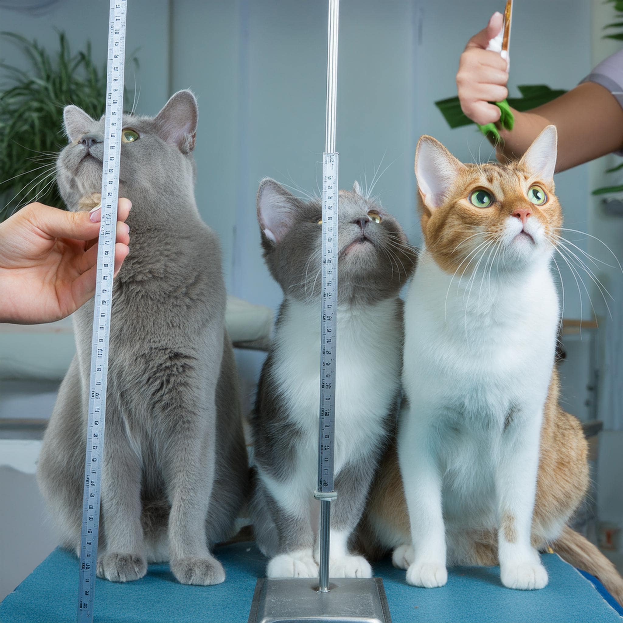 They are most interested in calculating the mean absolute deviation of the cat's heights to better understand how the sizes of the cats vary.
Finally, add the values found in the table and then divide the sum by the number of values, 12.
The mean absolute deviation is about 2.3 inches. This is the average distance of each data value from the mean. On average, the heights of cats deviate from the mean of 13 inches by about 2.3 inches.
 They are most interested in calculating the mean absolute deviation of the cat's heights to better understand how the sizes of the cats vary.
Height of Cats (in.)9, 9, 12, 15, 14, 11, 14, 15, 15, 10, 16, 16
Find the mean absolute deviation of the cat's heights. Round the answer to one decimal place. {"type":"text","form":{"type":"math","options":{"comparison":"1","nofractofloat":false,"keypad":{"simple":true,"useShortLog":false,"variables":["x"],"constants":["PI"]},"rendered":false},"text":"<span class=\"katex\"><span class=\"katex-html\" aria-hidden=\"true\"><\/span><\/span>"},"formTextBefore":null,"formTextAfter":"inches","answer":{"text":["2.3"]}}
Hint
Start by finding the mean. Then, calculate the distances between the mean and each data value. Finally, find the mean of these distances.
Solution
Begin by recalling what is the mean absolute deviation.
|
Mean Absolute Deviation |
|
An average of how much data values differ from the mean. |
To find the mean absolute deviation, these steps can be followed.
- Find the mean of the data
- Find the distance between each data value and the mean
- Find the average of the distances found in Step 2.
129, 9, 12, 15, 14, 11, 14, 15, 15, 10, 16, 16
The mean is a sum of all values divided by the number of them.
The mean of the data set is 13 inches. Now, move on to finding the distances between the data values and the mean. | Data Value | Absolute Value of Difference |
|---|---|
| 9 | ∣9−13∣=4 |
| 9 | ∣9−13∣=4 |
| 12 | ∣12−13∣=1 |
| 15 | ∣15−13∣=2 |
| 14 | ∣14−13∣=1 |
| 11 | ∣11−13∣=2 |
| 14 | ∣14−13∣=1 |
| 15 | ∣15−13∣=2 |
| 15 | ∣15−13∣=2 |
| 10 | ∣10−13∣=3 |
| 16 | ∣16−13∣=3 |
| 16 | ∣16−13∣=3 |
124+4+1+2+1+2+1+2+2+3+3+3
AddTerms
Add terms
1228
CalcQuot
Calculate quotient
2.333333…
RoundDec
Round to 1 decimal place(s)
≈2.3
Discussion
Standard Deviation
The standard deviation is a measure of spread of a data set that measures how much the data values differ from the mean. The Greek letter σ — read as 
 As illustrated, the standard deviation is the square root of the average of the squared differences between each value in the data set and the mean of the data set.
sigma— is commonly used to denote the standard deviation. In a given set of data, most of the values fall within one standard deviation of the mean.
Mean±Standard Deviation
For example, if the mean of a data set is 15 and the standard
deviation is 4, then most of the values fall between 11 and 19, as 15−4=11 and 15+4=19. Standard deviation shows the variation of data from the mean.
- If the standard deviation is small, it means the values in the data set are close to the mean.
- If the standard deviation is large, it means the values are spread out over a wider range.
Example
Data Values Beyond One Standard Deviation
Finally, Ignacio and Emily are examining the variation in the heights of dogs.
 Here are the values they are analyzing.
 Here are the values they are analyzing.
Height of Dogs (in.)24, 18, 22, 20, 26, 30, 28, 16, 25, 21
They found that the standard deviation of the heights is 4.2 inches. Which heights are not within one standard deviation from the mean? {"type":"text","form":{"type":"list","options":{"comparison":"1","nofractofloat":false,"keypad":{"simple":true,"useShortLog":false,"variables":["x"],"constants":["PI"]},"rendered":false,"ordermatters":false,"numinput":4,"listEditable":true,"hideNoSolution":true},"text":"<span class=\"katex\"><span class=\"katex-html\" aria-hidden=\"true\"><\/span><\/span>"},"formTextBefore":null,"formTextAfter":"inches","answer":{"text":["16","18","28","30"]}}
Hint
First find the mean of the given data set. Then, find the range of the values that are within one standard deviation from the mean.
Solution
Start by calculating the mean. The given data set consists of the heights of 10 dogs, measured in inches.

1024, 18, 22, 20, 26, 30, 28, 16, 25, 21
The mean is the sum of all values divided by the total number of values.
The mean of the data set is 23 inches. Now, find the range of values that are within one standard deviation of the mean! To do that, subtract one standard deviation from the mean and add one standard deviation to the mean — record both numbers. Mean−Standard Deviation=23−4.2=18.8Mean+Standard Deviation=23+4.2=27.2
The data values that are between 18.8 and 27.2 inches are within one standard deviation of the mean. The values that are less than 18.8 are 16 and 18, and the values that are greater than 27.2 are 28 and 30. That means the heights outside the range of one standard deviation from the mean are 16, 18, 28, and 30 inches.
Closure
Finding The Measures of Center of a Data Set
In this lesson, the measures of center and measures of spread were discussed.
| Measures of Center | Measures of Spread |
|---|---|
| Mean Mode Median |
Range Interquartile Range Mean Absolute Deviation Standard Deviation |
Lifespan of Cats (years)15,11,14,15,14,17,13
Remember that the mean of a data set is calculated by finding the sum of all values in the set and then dividing by the number of values in the set. Move the points to calculate the mean of the data set.


Loading content