
1-3. Quiz
Sign In
search
Exercise 8 Page 354
b Start by finding the outlier. Then calculate the measures of center without the outlier.
c Start by finding the five-number summary of the data.
d When each value of a data set is multiplied by a real number k>0, the measures of center and variation can be found by multiplying the original measures by k.
a Mean: $112
Median: $109.50
Mode: $98
Range: $116
b Outlier: $211
Mean: The outlier increases the mean by about $12.71.
Median: The outlier increases the median by $9.50.
c Box-and-Whisker Plot:
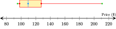
Interquartile Range: $29.50
Interquartile Range's Interpretation: The middle half of the prices vary by no more than 29.50.
d Mean: $115.90
Median: $104.025
Mode: $93.10
Range: $110.20
Practice makes perfect
a Consider the given table.
| Price (Dollars) | 98 | 119 | 95 | 211 | 130 | 98 | 100 | 125 |
|---|
The above table shows the prices of eight bikes in a sporting goods store. We are asked to find the measures of center and variability of the data. We will calculate each of them one at a time.
Mean
The mean of a numerical data set is the sum of the data divided by the number of data values. Since we have 8 values, we will divide the sum of the data by 8.x=Sum of Values/Number of Values
SubstituteValues
Substitute values
x=98+119+95+211+130+98+100+125/8
x=122
Median
The median of a numerical data set is the middle number when the values are written in numerical order. If the data set has an even number of values, the mean of the two middle values will be the median. Let's write the data in numerical order.95, 98, 98, 100, 119, 125, 130, 211 Since we have an even number of data values, the mean of the two middle values will be the median. Median:100+119/2=$109.50
Mode
The mode of a data set is the value or values that occur most often. Let's take a loot at our data. 95, 98, 98, 100, 119, 125, 130, 211 We can see that 98 is the value that occurs most often. Therefore, $98 is the mode.
Range
The range of a data set is the difference of the greatest value and the least value. In this case, the greatest value is $211 and the least value is $95. Range:$211-$95=$116
Standard Deviation
The standard deviation of a numerical data set is given by the following formula.
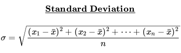
In this formula, n is the number of data values in the data set, x_1, x_2,..., x_n are the data values, and x_1-x, x_2-x,... x_n-x are the deviations of each data value. The deviation is given by the difference of the data value and the mean of the data set. We already found the mean of the data set. x=976/8 ⇒ x=$122 With this value we can calculate the deviation and the square of each deviation. Let's do this in a table.
| x | x | x-x | (x-x)^2 |
|---|---|---|---|
| 98 | 122 | -24 | 576 |
| 119 | 122 | -3 | 9 |
| 95 | 122 | -27 | 729 |
| 211 | 122 | 89 | 7921 |
| 130 | 122 | 8 | 64 |
| 98 | 122 | -24 | 576 |
| 100 | 122 | -22 | 484 |
| 125 | 122 | 3 | 9 |
b We are asked to find the outlier of the given data set. An outlier is a data value that is much greater than or much less than the other values in a data set. In this case, $211 is much greater than the other prices. Therefore, it is the outlier. To find out how this value affects the measures of center, let's analyze each measure one at a time.
Mean
Let's first remove the outlier from the given data. 98, 119, 95, 211, 130, 98, 100, 125 ⇓ 98, 119, 95, 130, 98, 100, 125 Since we have 7 data values, the mean will be the sum of the values divided by 7.x=Sum of Values/Number of Values
SubstituteValues
Substitute values
x=98+119+95+130+98+100+125/7
x≈ 109.29
Median
To find the mean after the outlier is removed, let's first write our data in numerical order. 95, 98, 98, 100, 119, 125, 130 In this case, the median is $100. Comparing it with the original median $109.5, we can see that the new median is less. Let's find the difference of these medians. $109.50-$100=$9.50 Therefore, the outlier increases the median by $9.50.
Mode
Again, let's take a look at the given values after the outlier is removed. 95, 98, 98, 100, 119, 125, 130 We can see that the mode is still $98. Therefore, the outlier does not affect the mode.
c To make a box-and-whisker plot of the data, let's first order the data to find the five-number summary.

Now, let's highlight this information in our ordered data.
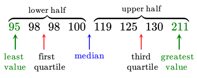
Let's draw a number line that includes the least and greatest value. Also, let's graph points above the number line for the five-number summary.
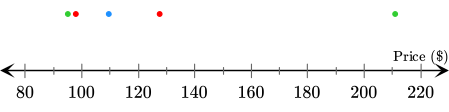
Finally, we can draw a box using Q_1 and Q_3. Then draw a line through the median and the whiskers from the box to the least and greatest values.
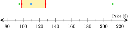
The interquartile range (IQR) is given by the difference of the third quartile, Q_3, and the first quartile, Q_1. It represents the range of the middle half of the data. We've found that Q_1 is 98 and Q_3 is 127.50. Let's calculate the difference of these values to find the interquartile range. Q_3- Q_1 ⇒ 127.5- 98=$29.50 This means that the middle half of the prices vary by no more than $29.50. Finally, we can see that the right whisker is longer than the left whisker, and most of the data are on the left side of the plot. Therefore, the distribution is skewed right.
d If the store offers 5 % of discount on all mountain bikes, by multiplying each old price by 95 % or 0.95 we will get the new prices. Additionally, when each value of a data set is multiplied by a real number k>0, the measures of center and variation can be found by multiplying the original measures by k. In this case, k is 0.95.
| Measure | Original Measures | * 0.95 | New Measures |
|---|---|---|---|
| Mean | 122 | 122 * 0.95 | 115.90 |
| Median | 109.50 | 109.50 * 0.95 | 104.025 |
| Mode | 98 | 98 * 0.95 | 93.10 |
| Range | 116 | 116 * 0.95 | 110.20 |
| Standard Deviation | 36 | 36 * 0.95 | 34.20 |
Loading content