{{ tocSubheader }}
{{ 'ml-label-loading-course' | message }}
An error ocurred, try again later!
Chapter {{ article.chapter.number }}
{{ article.number }}.
{{ article.displayTitle }}
{{ article.intro.summary }}
Show less Show more expand_more Lesson Settings & Tools
| | {{ 'ml-lesson-number-slides' | message : article.intro.bblockCount }} |
| | {{ 'ml-lesson-number-exercises' | message : article.intro.exerciseCount }} |
| | {{ 'ml-lesson-time-estimation' | message }} |
This lesson familiarizes the learner with how to summarize and display categorical data. Possible associations and trends will then be recognized by interpreting data from real-world examples.
Catch-Up and Review
Here are a few recommended readings before getting started with this lesson.
Challenge
Analyzing Data From a School Survey
Paulina loves dramas and wants to know what her classmates think about them. She decided to conduct a survey asking 50 students if they enjoy watching dramas. Paulina also noted if her classmates were 16 years and under or older than 16. Paulina wrote her findings in a notebook.
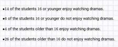
a How can these results be displayed in a single table?
b Is there an association between classmates who enjoying dramas and their age?
Discussion
Two-Way Frequency Tables, Joint and Marginal Frequencies
A two-way frequency table, also known as a two-way table, displays categorical data that can be grouped into two categories. One of the categories is represented in the rows of the table, the other in the columns. For example, the table below shows the results of a survey where 100 participants were asked if they have a driver's license and if they own a car.
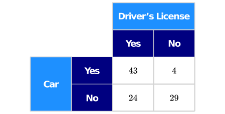
carand
driver's license.Both have possible responses of
yesand
no.The numbers in the table are called joint frequencies. Also, two-way frequency tables often include the total of the rows and columns — these are called marginal frequencies. Select any frequency in the table below to display more information.
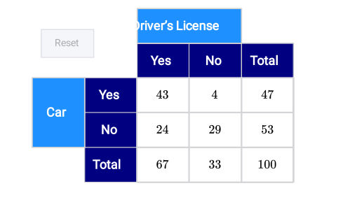
Totalrow and the
Totalcolumn, which in this case is 100, equals the sum of all joint frequencies. This is called the grand total. A joint frequency of 43 shows that 43 people have a driver's license and own a car. A marginal frequency of 53 shows that 53 people do not have a car. The rest of the numbers from the table can also be interpreted.
Discussion
Making a Two-Way Frequency Table
Organizing data in a two-way frequency table can help with visualization, which in turn makes it easier to analyze and present the data. To draw a two-way frequency table, three steps must be followed.
- Determine the categories.
- Fill the table with the given data.
- Determine if there are any missing frequencies. If so, find those.
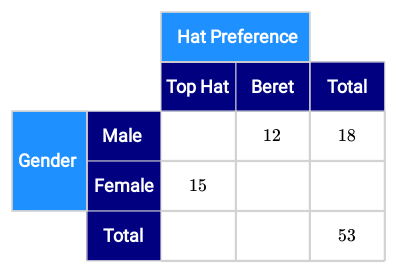
Suppose that 53 people took part in an online survey, where they were asked whether they prefer top hats or berets. Out of the 18 males that participated, 12 prefer berets. Also, 15 of the females chose top hats as their preference. The steps listed above will now be used to analyze and present the data.
1
Determine the Categories
expand_more First, the two categories of the table must be determined, after which the table can be drawn without frequencies. Here, the participants gave their hat preference and their gender, which are the two categories. Hat preference can be further divided into top hat and beret, and gender into female and male.
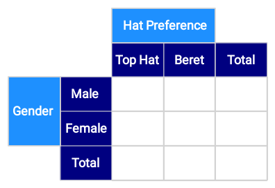
The total row and total column are included to write the marginal frequencies.
2
Fill the Table With Given Data
expand_more The given joint and marginal frequencies can now be added to the table.
3
Find Any Missing Frequencies
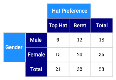
expand_more Using the given frequencies, more information can potentially be found by reasoning. For instance, because 12 out of the 18 males prefer berets, the number of males who prefer top hats is equal to the difference between these two values. 18 - 12 = 6 Therefore, there are 6 males who prefer top hats. Since there are 15 females who prefer top hats, the number of participants who prefer this type of hat is the sum of these two values. 6 + 15 = 21 It has been found that 21 participants prefer top hats. Continuing with this reasoning, the entire table can be completed.
Example
Night Owl or Early Bird?
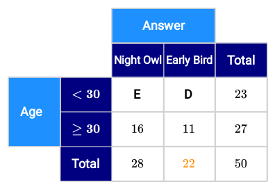
Zain has a job leading backpackers on excursions in the High Sierras. To better understand what time of day to plan certain activities, Zain posed a question to 50 backpackers about their sleep patterns: Are you a night owl or an early bird?
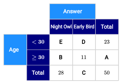
Zain then categorized the participants by sleep pattern and age — younger than 30 and 30 or older. Here is part of what was gathered.
- 11 people age 30 or older said they are early birds.
- 23 people younger than 30 participated in the survey.
- 28 people, of any age, said they are night owls.
Zain made a two-way frequency table with the data they collected. Unfortunately, some of the data values got smudged and are unable to be read! The missing data values have been replaced with letters, for now.
{"type":"pair","form":{"alts":[[{"id":0,"text":"A"},{"id":1,"text":"B"},{"id":2,"text":"C"},{"id":3,"text":"D"},{"id":4,"text":"E"}],[{"id":0,"text":"27"},{"id":1,"text":"16"},{"id":2,"text":"22"},{"id":3,"text":"11"},{"id":4,"text":"12"}]],"lockLeft":true,"lockRight":false},"formTextBefore":"","formTextAfter":"","answer":[[0,1,2,3,4],[0,1,2,3,4]]}
Hint
Begin by finding the number of people age 30 or older who participated in the survey. To do so, calculate the difference between the grand total and the number of participants younger than 30. That would be 50 divided by 23.
Solution
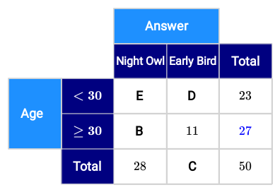
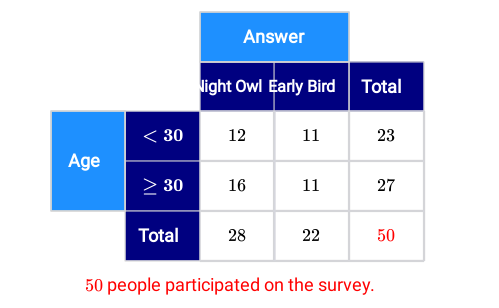
Start by finding the missing marginal frequency of the last column of the table, labeled A. Note that 50 people participated in the survey and 23 of them are younger than 30. Therefore, the number of participants who are 30 or older can be found by calculating the difference between these two values. 50-23= 27 This information can be added to the table.
With this information, the joint frequency B that represents the number of night owls aged 30 or older can be calculated. Of the 27 participants aged 30 or older, 11 are early birds. Therefore, the number of night owls aged 30 or older is the difference between these two values. 27-11= 16 This information can also be added to the table.

The missing marginal frequency C in the last row will now be calculated. Of the 50 participants, 28 said they are night owls. To find the number of early birds, the difference between these two values will be calculated. 50-28= 22 One more cell can be filled in!
Discussion
Joint and Marginal Relative Frequencies
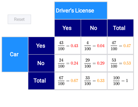
In a two-way frequency table, a joint relative frequency is the ratio of a joint frequency to the grand total. Similarly, a marginal relative frequency is the ratio of a marginal frequency to the grand total. Consider the following example of a two-way table.
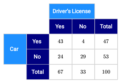
Here, the grand total is 100. The joint and marginal frequencies can now be divided by 100 to obtain the joint and marginal relative frequencies. Clicking in each cell will display its interpretation.
Example
Joint and Marginal Relative Frequencies for Night Owls and Early Birds
Previously, Zain made a two-way frequency table about backpackers sleep patterns.
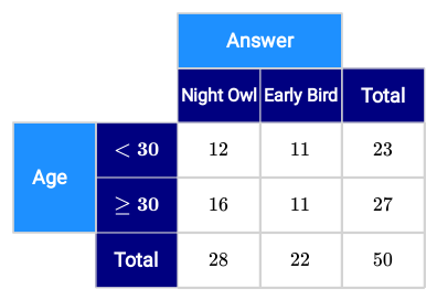
Zain wants to dig deeper into the data for even more clear interpretations, so they plan to calculate the joint and marginal relative frequencies.
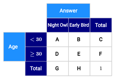
{"type":"pair","form":{"alts":[[{"id":0,"text":"A"},{"id":1,"text":"B"},{"id":2,"text":"C"},{"id":3,"text":"D"},{"id":4,"text":"E"},{"id":5,"text":"F"},{"id":6,"text":"G"},{"id":7,"text":"H"}],[{"id":0,"text":"0.24"},{"id":1,"text":"0.22"},{"id":2,"text":"0.46"},{"id":3,"text":"0.32"},{"id":4,"text":"0.22"},{"id":5,"text":"0.54"},{"id":6,"text":"0.56"},{"id":7,"text":"0.44"}]],"lockLeft":true,"lockRight":false},"formTextBefore":"","formTextAfter":"","answer":[[0,1,2,3,4,5,6,7],[0,1,2,3,4,5,6,7]]}
Solution
To calculate the joint and marginal relative frequencies, the joint and marginal frequencies must be divided by the grand total, 50.
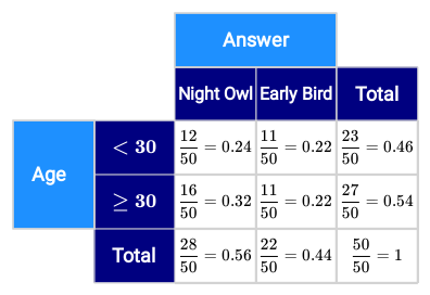
The table below shows the joint and marginal relative frequencies.
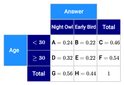
One finding — of a variety — based on the joint and marginal relative frequencies, shows that about one-third of the participants who are 30 or older are night owls. Additionally, Zain can see that the participants are almost equally distributed among the categories, as both pairs of marginal relative frequencies have values close to 50-50.
Discussion
Conditional Relative Frequency
A conditional relative frequency is the ratio of a joint frequency to either of its two corresponding marginal frequencies. Alternatively, it can be calculated using joint and marginal relative frequencies. As an example, the following data will be used.
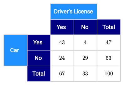
Referring to the column totals, the left column of joint frequencies should be divided by 67 and the right column by 33. Furthermore, since the column totals are used, the sum of the conditional relative frequencies of each column is 1.
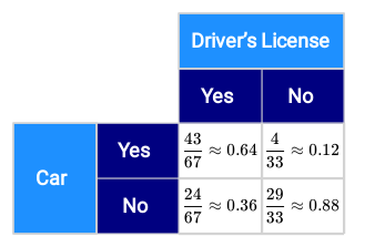
The resulting two-way frequency table can be interpreted to obtain the following information.
- Out of all the participants with a driver's license, about 64 % of them own a car.
- Out of all the participants with a driver's license, about 36 % of them do not own a car.
- Out of all the participants without a driver's license, about 12 % of them own a car.
- Out of all the participants without a driver's license, about 88 % of them do not own a car.
Example
Conditional Relative Frequencies for Night Owls and Early Birds
Using their two-way frequency table, Zain wants to continue improving the interpretation of their data by finding the conditional relative frequencies.
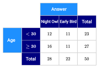
Zain will use the row totals to make the calculations.
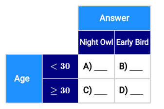
{"type":"pair","form":{"alts":[[{"id":0,"text":"A)"},{"id":1,"text":"B)"},{"id":2,"text":"C)"},{"id":3,"text":"D)"}],[{"id":0,"text":"\u2248 0.52"},{"id":1,"text":"\u2248 0.48"},{"id":2,"text":"\u2248 0.59"},{"id":3,"text":"\u2248 0.41"}]],"lockLeft":true,"lockRight":false},"formTextBefore":"","formTextAfter":"","answer":[[0,1,2,3],[0,1,2,3]]}
Hint
Since Zain uses the row totals, the joint frequencies in the first row must be divided by 23 and the joint frequencies in the second row must be divided by 27.
Solution
Zain uses the row totals. Therefore, the joint frequencies in the first row must be divided by 23 and the joint frequencies in the second row must be divided by 27.
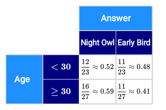
The table below shows the conditional relative frequencies.
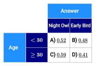
Extra
Applying Zain's Findings to an Actual Backpacking TripZain interprets the various findings as reason to believe when planning night activities, like storytelling over a campfire, they could tailor the stories for an older generation. Interestingly, the older backpackers, as a whole, seem to prefer nights more than the younger backpackers. Zain can now plan according to these interpretations.
Discussion
Looking for Associations in Data
How to make two-way frequency tables and interpret the information presented in those tables has been shown. Next, how to recognize associations in data that come from a two-way table will be discussed.
Method
Recognizing Associations in Data
Studying the conditional relative frequencies of a two-way frequency table, it is possible to find potential associations in the data. As an example, the following survey results will be analyzed.
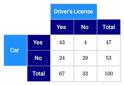
First, the conditional relative frequencies can be found by dividing each joint frequency by the corresponding column's marginal frequency.
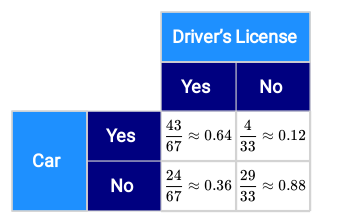
As can be seen, 64% of people with a driver's license own a car, while 88% of people without a drivers license do not own a car. Therefore, an association between having a driver's license and owning a car might exist. On the other hand, finding the conditional relative frequencies using the row's marginal frequencies gives a slightly different result.
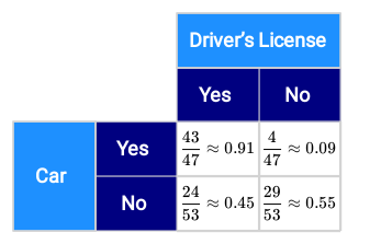
As can be seen, among car owners, almost everyone has a driver's license. Meanwhile, among the people who do not own a car, roughly half have a driver's license. This observation shows that car ownership is associated with having a driver's license, while not owning a car is not associated with not having a driver's license. Car &⇒ Driver's license ✓ No car & ⇒ No driver's license * Consider a different two-way frequency table that illustrates a stronger association when using the marginal frequencies of only one variable.
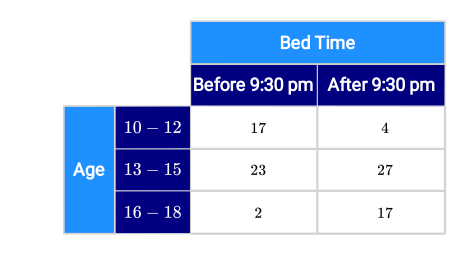
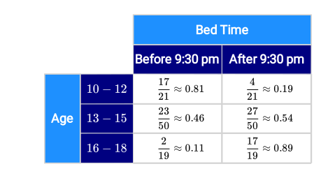
A person's bed time might be dependent on their age, but their age is not dependent on their bed time. Because of this, it is recommended to use the age's marginal frequencies when finding the conditional relative frequencies. This gives the distribution of bed time given a certain age span.
Closure
Determining Associations From a Survey's Data
The challenge at the beginning of this lesson showed the following information that Paulina gathered when she conducted a survey at her school.
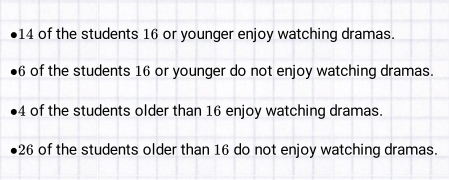
The following challenge questions were then asked.
a How can these results be displayed in a single table?
b Is there an association between a student enjoying watching dramas and their age?
Answer
a 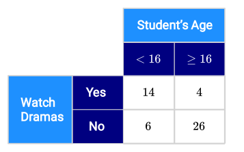
b Yes, younger students are more likely to watch dramas.
Hint
a Use a two-way frequency table.
b Analyze the conditional relative frequencies.
Solution
a A two-way frequency table can be used to display the given information using a single table. Whether the students enjoy dramas or not and their age ranges can be chosen as the two main categories of the table. The data Paula collected can then be entered into the appropriate cells.
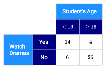
b The conditional relative frequencies of the data can be found and analyzed to help determine if the data values are related. Begin by calculating the marginal frequencies. Add the joint frequencies of each row and each column of the table to the Total's row and column, respectively.
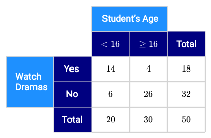
First, focus on the cells related directly to the student's age. There are 20 students under the age of 16 and there are 30 students who are 16 or older. These marginal frequency totals occur regardless of the student's interest in dramas.
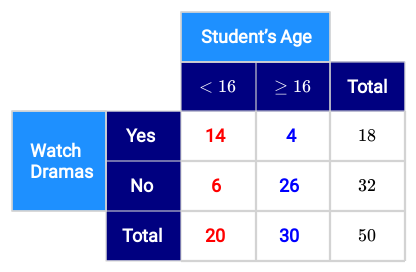
Next, divide each joint frequency by the corresponding marginal frequency related to age.
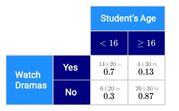
The table shows that 70% of the students 16 years old or younger watch dramas. Whereas, only 13% of the students older than 16 watch dramas. A similar analysis can be done with the marginal frequencies according to the Yes
or No
rows.
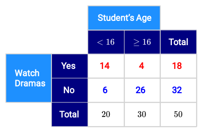
Using the marginal frequencies of 18 and 32, make the necessary calculations.
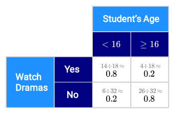
The results indicate that there are associations between watching dramas and a student's age. It is seen that 80% of the students under 16 watch dramas. Whereas, 80% of students 16 or older do not watch dramas.
While Paula feels excellent about her interpretations of the data, she knows that these associations are limited to this survey's sample. Her interpretations apply only to her classmates who joined the survey, not how everyone at the school feels about dramas.
Loading content