Reference

Normal Distribution

Concept

Normal Distribution

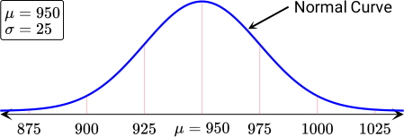
A normal distribution is a type of probability distribution where the mean, the median, and the mode are all equal to each other. The graph that represents a normal distribution is called a normal curve and it is a continuous, bell-shaped curve that is symmetric with respect to the mean μ of the data set.

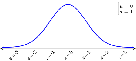
This type of distribution is the most common continuous probability distribution that can be observed in real life. When a normal distribution has a mean of 0 and standard deviation of 1, it is called a standard normal distribution. A normal distribution can be standardized by transforming each of its values into their corresponding z-scores.

The total area under the normal curve is 100 %, or 1. Because of this, the area under the normal curve in a certain interval represents the percentage of data within that interval or the probability of randomly selecting a value that belongs to that interval. The Empirical Rule can be used to determine the area under the normal curve at specific intervals.

Example

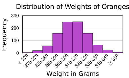
Consider the weights of oranges as an example of normally distributed data. The mean weight of an orange is about 310 grams and the standard deviation is approximately 15 grams. The distribution of a sample of weights of 1000 randomly chosen oranges is described by the following histogram.

The histogram will look more and more like a normal curve as more and more observations are made. In addition to this example, topics such as human height or income also tend to be normally distributed. It is also worth noting that not all data sets are normally distributed. If the mean and median are not equal, then the data set is skewed.

Concept

Empirical Rule

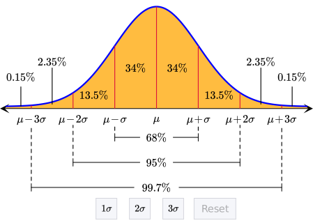
In statistics, the Empirical Rule, also known as the 68–95–99.7 rule, is a shorthand used to remember the percentage of values that lie within certain intervals in a normal distribution. The rule states the following three facts.

About 68 % of the values lie within one standard deviation of the mean.
About 95 % of the values lie within two standard deviations of the mean.
About 99.7 % of the values lie within three standard deviations of the mean.

These three facts can be confirmed by observing the area under the normal curve that corresponds to a normal distribution with mean μ and standard deviation σ.

According to this rule, almost all the values observed lie within three standard deviations of the mean. For this reason, the rule is also called the three-sigma rule. It is worth noting that these facts were observed based on empirical evidence, which is why it is called the Empirical Rule.

Concept

z-Score

The z-score, also known as the z-value, represents the number of standard deviations that a given value x is from the mean of a data set. The following formula can be used to convert any x-value into its corresponding z-score.

z=x-μ/σ

Here, μ represents the mean and σ the standard deviation of the distribution. The z-value corresponding to a sample mean x is called a z-statistic and is calculated using a similar formula.

z=x-μ/ssqrt(n)

In this formula, s is the standard deviation of the sample, n is the sample size, and μ is the population mean.

Example

Consider a distribution with mean 12 and standard deviation 2.5. The z-score corresponding to x=11.5 is computed as follows. z = 11.5-12/2.5 ⇔ z = -0.2

Consequently, 11.5 is 0.2 standard deviations to the left of the mean. The z-scores can be used to standardize a normal distribution. Then, for a random z-value of a standard normal distribution, the Standard Normal Table can be used to determine the corresponding area under the curve.

Memo

Standard Normal Table

The left-hand column gives the whole part of z, while the top row gives the decimal part of z.

	.0	.1	.2	.3	.4	.5	.6	.7	.8	.9
-3	.00135	.00097	.00069	.00048	.00034	.00023	.00016	.00011	.00007	.00005
-2	.02275	.01786	.01390	.01072	.00820	.00621	.00466	.00347	.00256	.00187
-1	.15866	.13567	.11507	.09680	.08076	.06681	.05480	.04457	.03593	.02872
-0	.50000	.46017	.42074	.38209	.34458	.30854	.27425	.24196	.21186	.18406
0	.50000	.53983	.57926	.61791	.65542	.69146	.72575	.75804	.78814	.81594
1	.84134	.86433	.88493	.90320	.91924	.93319	.94520	.95543	.96407	.97128
2	.97725	.98214	.98610	.98928	.99180	.99379	.99534	.99653	.99744	.99813
3	.99865	.99903	.99931	.99952	.99966	.99977	.99984	.99989	.99993	.99995

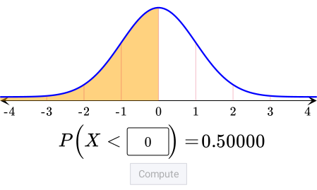
The applet calculates the area below the standard normal curve and to the left of the entered z-score. It accepts z-scores up to two decimal places.

Example

Example

Recommended exercises